Learning Rate Scheduling
Run Jupyter Notebook
You can run the code for this section in this jupyter notebook link.
Optimization Algorithm: Mini-batch Stochastic Gradient Descent (SGD)
- We will be using mini-batch gradient descent in all our examples here when scheduling our learning rate
- Combination of batch gradient descent & stochastic gradient descent
- \(\theta = \theta - \eta \cdot \nabla J(\theta, x^{i: i+n}, y^{i:i+n})\)
- Characteristics
- Compute the gradient of the lost function w.r.t. parameters for n sets of training sample (n input and n label), \(\nabla J(\theta, x^{i: i+n}, y^{i:i+n})\)
- Use this to update our parameters at every iteration
- Typically in deep learning, some variation of mini-batch gradient is used where the batch size is a hyperparameter to be determined
Learning Intuition Recap
- Learning process
- Original parameters \(\rightarrow\) given input, get output \(\rightarrow\) compare with labels \(\rightarrow\) get loss with comparison of input/output \(\rightarrow\) get gradients of loss w.r.t parameters \(\rightarrow\) update parameters so model can churn output closer to labels \(\rightarrow\) repeat
- For a detailed mathematical account of how this works and how to implement from scratch in Python and PyTorch, you can read our forward- and back-propagation and gradient descent post.
Learning Rate Pointers
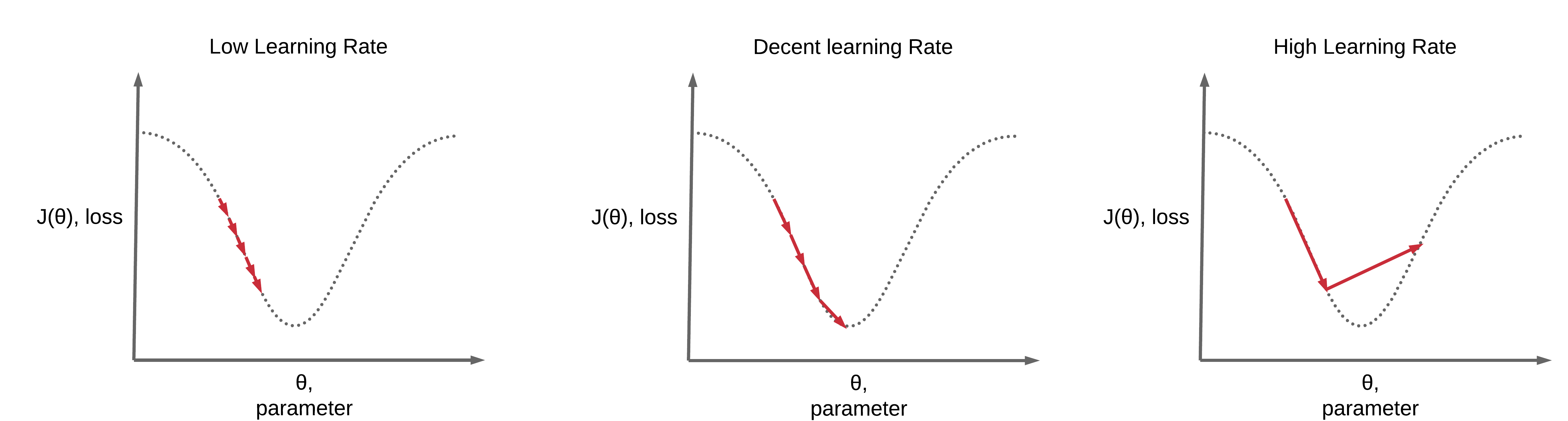
- Update parameters so model can churn output closer to labels, lower loss
- \(\theta = \theta - \eta \cdot \nabla J(\theta, x^{i: i+n}, y^{i:i+n})\)
- If we set \(\eta\) to be a large value \(\rightarrow\) learn too much (rapid learning)
- Unable to converge to a good local minima (unable to effectively gradually decrease your loss, overshoot the local lowest value)
- If we set \(\eta\) to be a small value \(\rightarrow\) learn too little (slow learning)
- May take too long or unable to converge to a good local minima
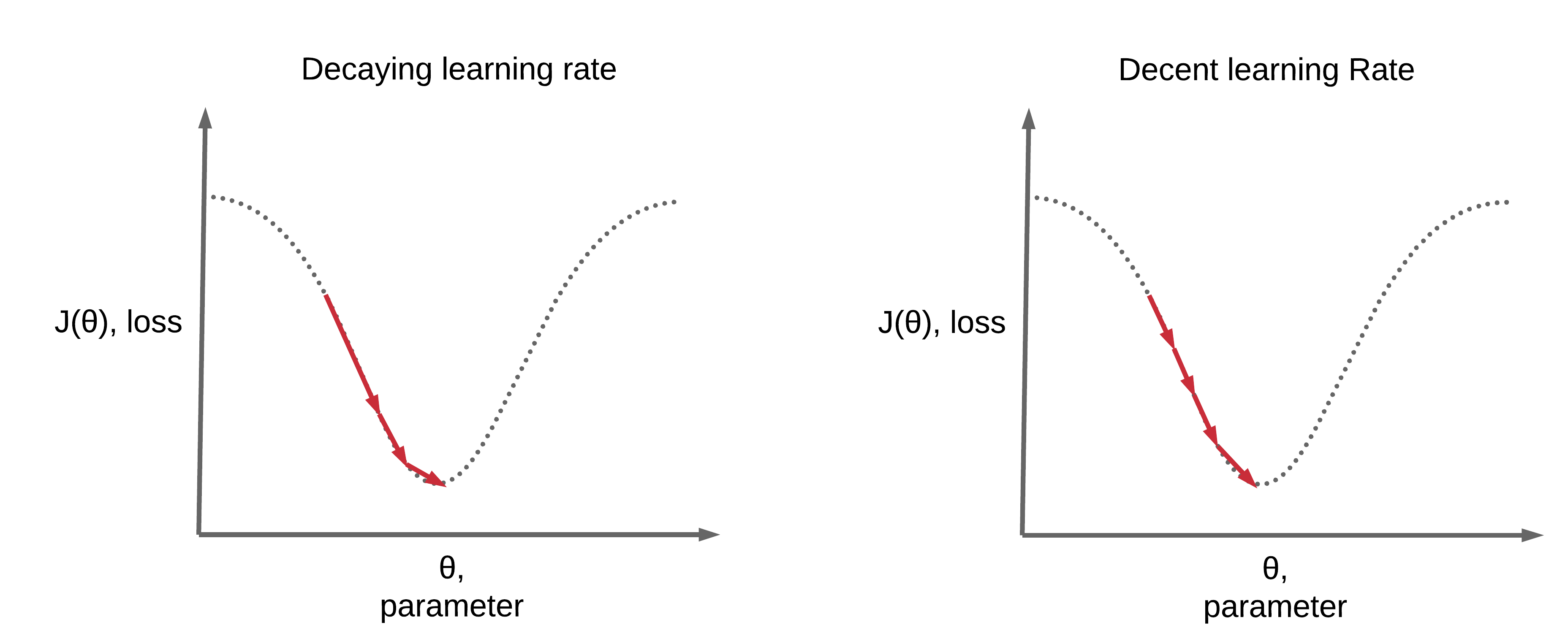
Need for Learning Rate Schedules
- Benefits
- Converge faster
- Higher accuracy
Top Basic Learning Rate Schedules
- Step-wise Decay
- Reduce on Loss Plateau Decay
Step-wise Learning Rate Decay
Step-wise Decay: Every Epoch
- At every epoch,
- \(\eta_t = \eta_{t-1}\gamma\)
- \(\gamma = 0.1\)
- Optimization Algorithm 4: SGD Nesterov
- Modification of SGD Momentum
- \(v_t = \gamma v_{t-1} + \eta \cdot \nabla J(\theta - \gamma v_{t-1}, x^{i: i+n}, y^{i:i+n})\)
- \(\theta = \theta - v_t\)
- Modification of SGD Momentum
- Practical example
- Given \(\eta_t = 0.1\) and $ \gamma = 0.01$
- Epoch 0: \(\eta_t = 0.1\)
- Epoch 1: \(\eta_{t+1} = 0.1 (0.1) = 0.01\)
- Epoch 2: \(\eta_{t+2} = 0.1 (0.1)^2 = 0.001\)
- Epoch n: \(\eta_{t+n} = 0.1 (0.1)^n\)
Code for step-wise learning rate decay at every epoch
import torch
import torch.nn as nn
import torchvision.transforms as transforms
import torchvision.datasets as dsets

# Set seed
torch.manual_seed(0)

# Where to add a new import
from torch.optim.lr_scheduler import StepLR

'''
STEP 1: LOADING DATASET
'''

train_dataset = dsets.MNIST(root='./data',
                            train=True,
                            transform=transforms.ToTensor(),
                            download=True)

test_dataset = dsets.MNIST(root='./data',
                           train=False,
                           transform=transforms.ToTensor())

'''
STEP 2: MAKING DATASET ITERABLE
'''

batch_size = 100
n_iters = 3000
num_epochs = n_iters / (len(train_dataset) / batch_size)
num_epochs = int(num_epochs)

train_loader = torch.utils.data.DataLoader(dataset=train_dataset,
                                           batch_size=batch_size,
                                           shuffle=True)

test_loader = torch.utils.data.DataLoader(dataset=test_dataset,
                                          batch_size=batch_size,
                                          shuffle=False)

'''
STEP 3: CREATE MODEL CLASS
'''
class FeedforwardNeuralNetModel(nn.Module):
    def __init__(self, input_dim, hidden_dim, output_dim):
        super(FeedforwardNeuralNetModel, self).__init__()
        # Linear function
        self.fc1 = nn.Linear(input_dim, hidden_dim)
        # Non-linearity
        self.relu = nn.ReLU()
        # Linear function (readout)
        self.fc2 = nn.Linear(hidden_dim, output_dim)

    def forward(self, x):
        # Linear function
        out = self.fc1(x)
        # Non-linearity
        out = self.relu(out)
        # Linear function (readout)
        out = self.fc2(out)
        return out
'''
STEP 4: INSTANTIATE MODEL CLASS
'''
input_dim = 28*28
hidden_dim = 100
output_dim = 10

model = FeedforwardNeuralNetModel(input_dim, hidden_dim, output_dim)

'''
STEP 5: INSTANTIATE LOSS CLASS
'''
criterion = nn.CrossEntropyLoss()


'''
STEP 6: INSTANTIATE OPTIMIZER CLASS
'''
learning_rate = 0.1

optimizer = torch.optim.SGD(model.parameters(), lr=learning_rate, momentum=0.9, nesterov=True)

'''
STEP 7: INSTANTIATE STEP LEARNING SCHEDULER CLASS
'''
# step_size: at how many multiples of epoch you decay
# step_size = 1, after every 1 epoch, new_lr = lr*gamma
# step_size = 2, after every 2 epoch, new_lr = lr*gamma

# gamma = decaying factor
scheduler = StepLR(optimizer, step_size=1, gamma=0.1)

'''
STEP 7: TRAIN THE MODEL
'''
iter = 0
for epoch in range(num_epochs):
    # Decay Learning Rate
    scheduler.step()
    # Print Learning Rate
    print('Epoch:', epoch,'LR:', scheduler.get_lr())
    for i, (images, labels) in enumerate(train_loader):
        # Load images
        images = images.view(-1, 28*28).requires_grad_()

        # Clear gradients w.r.t. parameters
        optimizer.zero_grad()

        # Forward pass to get output/logits
        outputs = model(images)

        # Calculate Loss: softmax --> cross entropy loss
        loss = criterion(outputs, labels)

        # Getting gradients w.r.t. parameters
        loss.backward()

        # Updating parameters
        optimizer.step()

        iter += 1

        if iter % 500 == 0:
            # Calculate Accuracy
            correct = 0
            total = 0
            # Iterate through test dataset
            for images, labels in test_loader:
                # Load images to a Torch Variable
                images = images.view(-1, 28*28)

                # Forward pass only to get logits/output
                outputs = model(images)

                # Get predictions from the maximum value
                _, predicted = torch.max(outputs.data, 1)

                # Total number of labels
                total += labels.size(0)

                # Total correct predictions
                correct += (predicted == labels).sum()

            accuracy = 100 * correct / total

            # Print Loss
            print('Iteration: {}. Loss: {}. Accuracy: {}'.format(iter, loss.item(), accuracy))
Epoch: 0 LR: [0.1]
Iteration: 500. Loss: 0.15292978286743164. Accuracy: 96
Epoch: 1 LR: [0.010000000000000002]
Iteration: 1000. Loss: 0.1207798570394516. Accuracy: 97
Epoch: 2 LR: [0.0010000000000000002]
Iteration: 1500. Loss: 0.12287932634353638. Accuracy: 97
Epoch: 3 LR: [0.00010000000000000003]
Iteration: 2000. Loss: 0.05614742264151573. Accuracy: 97
Epoch: 4 LR: [1.0000000000000003e-05]
Iteration: 2500. Loss: 0.06775809079408646. Accuracy: 97
Iteration: 3000. Loss: 0.03737065941095352. Accuracy: 97
Step-wise Decay: Every 2 Epochs
- At every 2 epoch,
- \(\eta_t = \eta_{t-1}\gamma\)
- \(\gamma = 0.1\)
- Optimization Algorithm 4: SGD Nesterov
- Modification of SGD Momentum
- \(v_t = \gamma v_{t-1} + \eta \cdot \nabla J(\theta - \gamma v_{t-1}, x^{i: i+n}, y^{i:i+n})\)
- \(\theta = \theta - v_t\)
- Modification of SGD Momentum
- Practical example
- Given \(\eta_t = 0.1\) and \(\gamma = 0.01\)
- Epoch 0: \(\eta_t = 0.1\)
- Epoch 1: \(\eta_{t+1} = 0.1\)
- Epoch 2: \(\eta_{t+2} = 0.1 (0.1) = 0.01\)
Code for step-wise learning rate decay at every 2 epoch
import torch
import torch.nn as nn
import torchvision.transforms as transforms
import torchvision.datasets as dsets

# Set seed
torch.manual_seed(0)

# Where to add a new import
from torch.optim.lr_scheduler import StepLR

'''
STEP 1: LOADING DATASET
'''

train_dataset = dsets.MNIST(root='./data',
                            train=True,
                            transform=transforms.ToTensor(),
                            download=True)

test_dataset = dsets.MNIST(root='./data',
                           train=False,
                           transform=transforms.ToTensor())

'''
STEP 2: MAKING DATASET ITERABLE
'''

batch_size = 100
n_iters = 3000
num_epochs = n_iters / (len(train_dataset) / batch_size)
num_epochs = int(num_epochs)

train_loader = torch.utils.data.DataLoader(dataset=train_dataset,
                                           batch_size=batch_size,
                                           shuffle=True)

test_loader = torch.utils.data.DataLoader(dataset=test_dataset,
                                          batch_size=batch_size,
                                          shuffle=False)

'''
STEP 3: CREATE MODEL CLASS
'''
class FeedforwardNeuralNetModel(nn.Module):
    def __init__(self, input_dim, hidden_dim, output_dim):
        super(FeedforwardNeuralNetModel, self).__init__()
        # Linear function
        self.fc1 = nn.Linear(input_dim, hidden_dim)
        # Non-linearity
        self.relu = nn.ReLU()
        # Linear function (readout)
        self.fc2 = nn.Linear(hidden_dim, output_dim)

    def forward(self, x):
        # Linear function
        out = self.fc1(x)
        # Non-linearity
        out = self.relu(out)
        # Linear function (readout)
        out = self.fc2(out)
        return out
'''
STEP 4: INSTANTIATE MODEL CLASS
'''
input_dim = 28*28
hidden_dim = 100
output_dim = 10

model = FeedforwardNeuralNetModel(input_dim, hidden_dim, output_dim)

'''
STEP 5: INSTANTIATE LOSS CLASS
'''
criterion = nn.CrossEntropyLoss()

'''
STEP 6: INSTANTIATE OPTIMIZER CLASS
'''
learning_rate = 0.1

optimizer = torch.optim.SGD(model.parameters(), lr=learning_rate, momentum=0.9, nesterov=True)

'''
STEP 7: INSTANTIATE STEP LEARNING SCHEDULER CLASS
'''
# step_size: at how many multiples of epoch you decay
# step_size = 1, after every 2 epoch, new_lr = lr*gamma
# step_size = 2, after every 2 epoch, new_lr = lr*gamma

# gamma = decaying factor
scheduler = StepLR(optimizer, step_size=2, gamma=0.1)

'''
STEP 7: TRAIN THE MODEL
'''
iter = 0
for epoch in range(num_epochs):
    # Decay Learning Rate
    scheduler.step()
    # Print Learning Rate
    print('Epoch:', epoch,'LR:', scheduler.get_lr())
    for i, (images, labels) in enumerate(train_loader):
        # Load images as Variable
        images = images.view(-1, 28*28).requires_grad_()

        # Clear gradients w.r.t. parameters
        optimizer.zero_grad()

        # Forward pass to get output/logits
        outputs = model(images)

        # Calculate Loss: softmax --> cross entropy loss
        loss = criterion(outputs, labels)

        # Getting gradients w.r.t. parameters
        loss.backward()

        # Updating parameters
        optimizer.step()

        iter += 1

        if iter % 500 == 0:
            # Calculate Accuracy
            correct = 0
            total = 0
            # Iterate through test dataset
            for images, labels in test_loader:
                # Load images to a Torch Variable
                images = images.view(-1, 28*28).requires_grad_()

                # Forward pass only to get logits/output
                outputs = model(images)

                # Get predictions from the maximum value
                _, predicted = torch.max(outputs.data, 1)

                # Total number of labels
                total += labels.size(0)

                # Total correct predictions
                correct += (predicted == labels).sum()

            accuracy = 100 * correct / total

            # Print Loss
            print('Iteration: {}. Loss: {}. Accuracy: {}'.format(iter, loss.item(), accuracy))
Epoch: 0 LR: [0.1]
Iteration: 500. Loss: 0.15292978286743164. Accuracy: 96
Epoch: 1 LR: [0.1]
Iteration: 1000. Loss: 0.11253029108047485. Accuracy: 96
Epoch: 2 LR: [0.010000000000000002]
Iteration: 1500. Loss: 0.14498558640480042. Accuracy: 97
Epoch: 3 LR: [0.010000000000000002]
Iteration: 2000. Loss: 0.03691177815198898. Accuracy: 97
Epoch: 4 LR: [0.0010000000000000002]
Iteration: 2500. Loss: 0.03511016443371773. Accuracy: 97
Iteration: 3000. Loss: 0.029424520209431648. Accuracy: 97
Step-wise Decay: Every Epoch, Larger Gamma
- At every epoch,
- \(\eta_t = \eta_{t-1}\gamma\)
- \(\gamma = 0.96\)
- Optimization Algorithm 4: SGD Nesterov
- Modification of SGD Momentum
- \(v_t = \gamma v_{t-1} + \eta \cdot \nabla J(\theta - \gamma v_{t-1}, x^{i: i+n}, y^{i:i+n})\)
- \(\theta = \theta - v_t\)
- Modification of SGD Momentum
- Practical example
- Given \(\eta_t = 0.1\) and \(\gamma = 0.96\)
- Epoch 1: \(\eta_t = 0.1\)
- Epoch 2: \(\eta_{t+1} = 0.1 (0.96) = 0.096\)
- Epoch 3: \(\eta_{t+2} = 0.1 (0.96)^2 = 0.092\)
- Epoch n: \(\eta_{t+n} = 0.1 (0.96)^n\)
Code for step-wise learning rate decay at every epoch with larger gamma
import torch
import torch.nn as nn
import torchvision.transforms as transforms
import torchvision.datasets as dsets

# Set seed
torch.manual_seed(0)

# Where to add a new import
from torch.optim.lr_scheduler import StepLR

'''
STEP 1: LOADING DATASET
'''

train_dataset = dsets.MNIST(root='./data',
                            train=True,
                            transform=transforms.ToTensor(),
                            download=True)

test_dataset = dsets.MNIST(root='./data',
                           train=False,
                           transform=transforms.ToTensor())

'''
STEP 2: MAKING DATASET ITERABLE
'''

batch_size = 100
n_iters = 3000
num_epochs = n_iters / (len(train_dataset) / batch_size)
num_epochs = int(num_epochs)

train_loader = torch.utils.data.DataLoader(dataset=train_dataset,
                                           batch_size=batch_size,
                                           shuffle=True)

test_loader = torch.utils.data.DataLoader(dataset=test_dataset,
                                          batch_size=batch_size,
                                          shuffle=False)

'''
STEP 3: CREATE MODEL CLASS
'''
class FeedforwardNeuralNetModel(nn.Module):
    def __init__(self, input_dim, hidden_dim, output_dim):
        super(FeedforwardNeuralNetModel, self).__init__()
        # Linear function
        self.fc1 = nn.Linear(input_dim, hidden_dim)
        # Non-linearity
        self.relu = nn.ReLU()
        # Linear function (readout)
        self.fc2 = nn.Linear(hidden_dim, output_dim)

    def forward(self, x):
        # Linear function
        out = self.fc1(x)
        # Non-linearity
        out = self.relu(out)
        # Linear function (readout)
        out = self.fc2(out)
        return out
'''
STEP 4: INSTANTIATE MODEL CLASS
'''
input_dim = 28*28
hidden_dim = 100
output_dim = 10

model = FeedforwardNeuralNetModel(input_dim, hidden_dim, output_dim)

'''
STEP 5: INSTANTIATE LOSS CLASS
'''
criterion = nn.CrossEntropyLoss()


'''
STEP 6: INSTANTIATE OPTIMIZER CLASS
'''
learning_rate = 0.1

optimizer = torch.optim.SGD(model.parameters(), lr=learning_rate, momentum=0.9, nesterov=True)

'''
STEP 7: INSTANTIATE STEP LEARNING SCHEDULER CLASS
'''
# step_size: at how many multiples of epoch you decay
# step_size = 1, after every 2 epoch, new_lr = lr*gamma
# step_size = 2, after every 2 epoch, new_lr = lr*gamma

# gamma = decaying factor
scheduler = StepLR(optimizer, step_size=2, gamma=0.96)

'''
STEP 7: TRAIN THE MODEL
'''
iter = 0
for epoch in range(num_epochs):
    # Decay Learning Rate
    scheduler.step()
    # Print Learning Rate
    print('Epoch:', epoch,'LR:', scheduler.get_lr())
    for i, (images, labels) in enumerate(train_loader):
        # Load images as Variable
        images = images.view(-1, 28*28).requires_grad_()

        # Clear gradients w.r.t. parameters
        optimizer.zero_grad()

        # Forward pass to get output/logits
        outputs = model(images)

        # Calculate Loss: softmax --> cross entropy loss
        loss = criterion(outputs, labels)

        # Getting gradients w.r.t. parameters
        loss.backward()

        # Updating parameters
        optimizer.step()

        iter += 1

        if iter % 500 == 0:
            # Calculate Accuracy
            correct = 0
            total = 0
            # Iterate through test dataset
            for images, labels in test_loader:
                # Load images to a Torch Variable
                images = images.view(-1, 28*28)

                # Forward pass only to get logits/output
                outputs = model(images)

                # Get predictions from the maximum value
                _, predicted = torch.max(outputs.data, 1)

                # Total number of labels
                total += labels.size(0)

                # Total correct predictions
                correct += (predicted == labels).sum()

            accuracy = 100 * correct / total

            # Print Loss
            print('Iteration: {}. Loss: {}. Accuracy: {}'.format(iter, loss.item(), accuracy))
Epoch: 0 LR: [0.1]
Iteration: 500. Loss: 0.15292978286743164. Accuracy: 96
Epoch: 1 LR: [0.1]
Iteration: 1000. Loss: 0.11253029108047485. Accuracy: 96
Epoch: 2 LR: [0.096]
Iteration: 1500. Loss: 0.11864850670099258. Accuracy: 97
Epoch: 3 LR: [0.096]
Iteration: 2000. Loss: 0.030942382290959358. Accuracy: 97
Epoch: 4 LR: [0.09216]
Iteration: 2500. Loss: 0.04521659016609192. Accuracy: 97
Iteration: 3000. Loss: 0.027839098125696182. Accuracy: 97
Pointers on Step-wise Decay
- You would want to decay your LR gradually when you're training more epochs
- Converge too fast, to a crappy loss/accuracy, if you decay rapidly
- To decay slower
- Larger \(\gamma\)
- Larger interval of decay
Reduce on Loss Plateau Decay
Reduce on Loss Plateau Decay, Patience=0, Factor=0.1
- Reduce learning rate whenever loss plateaus
- Patience: number of epochs with no improvement after which learning rate will be reduced
- Patience = 0
- Factor: multiplier to decrease learning rate, \(lr = lr*factor = \gamma\)
- Factor = 0.1
- Patience: number of epochs with no improvement after which learning rate will be reduced
- Optimization Algorithm: SGD Nesterov
- Modification of SGD Momentum
- \(v_t = \gamma v_{t-1} + \eta \cdot \nabla J(\theta - \gamma v_{t-1}, x^{i: i+n}, y^{i:i+n})\)
- \(\theta = \theta - v_t\)
- Modification of SGD Momentum
Code for reduce on loss plateau learning rate decay of factor 0.1 and 0 patience
import torch
import torch.nn as nn
import torchvision.transforms as transforms
import torchvision.datasets as dsets

# Set seed
torch.manual_seed(0)

# Where to add a new import
from torch.optim.lr_scheduler import ReduceLROnPlateau

'''
STEP 1: LOADING DATASET
'''

train_dataset = dsets.MNIST(root='./data',
                            train=True,
                            transform=transforms.ToTensor(),
                            download=True)

test_dataset = dsets.MNIST(root='./data',
                           train=False,
                           transform=transforms.ToTensor())

'''
STEP 2: MAKING DATASET ITERABLE
'''

batch_size = 100
n_iters = 6000
num_epochs = n_iters / (len(train_dataset) / batch_size)
num_epochs = int(num_epochs)

train_loader = torch.utils.data.DataLoader(dataset=train_dataset,
                                           batch_size=batch_size,
                                           shuffle=True)

test_loader = torch.utils.data.DataLoader(dataset=test_dataset,
                                          batch_size=batch_size,
                                          shuffle=False)

'''
STEP 3: CREATE MODEL CLASS
'''
class FeedforwardNeuralNetModel(nn.Module):
    def __init__(self, input_dim, hidden_dim, output_dim):
        super(FeedforwardNeuralNetModel, self).__init__()
        # Linear function
        self.fc1 = nn.Linear(input_dim, hidden_dim)
        # Non-linearity
        self.relu = nn.ReLU()
        # Linear function (readout)
        self.fc2 = nn.Linear(hidden_dim, output_dim)

    def forward(self, x):
        # Linear function
        out = self.fc1(x)
        # Non-linearity
        out = self.relu(out)
        # Linear function (readout)
        out = self.fc2(out)
        return out
'''
STEP 4: INSTANTIATE MODEL CLASS
'''
input_dim = 28*28
hidden_dim = 100
output_dim = 10

model = FeedforwardNeuralNetModel(input_dim, hidden_dim, output_dim)

'''
STEP 5: INSTANTIATE LOSS CLASS
'''
criterion = nn.CrossEntropyLoss()


'''
STEP 6: INSTANTIATE OPTIMIZER CLASS
'''
learning_rate = 0.1

optimizer = torch.optim.SGD(model.parameters(), lr=learning_rate, momentum=0.9, nesterov=True)

'''
STEP 7: INSTANTIATE STEP LEARNING SCHEDULER CLASS
'''
# lr = lr * factor
# mode='max': look for the maximum validation accuracy to track
# patience: number of epochs - 1 where loss plateaus before decreasing LR
        # patience = 0, after 1 bad epoch, reduce LR
# factor = decaying factor
scheduler = ReduceLROnPlateau(optimizer, mode='max', factor=0.1, patience=0, verbose=True)

'''
STEP 7: TRAIN THE MODEL
'''
iter = 0
for epoch in range(num_epochs):
    for i, (images, labels) in enumerate(train_loader):
        # Load images as Variable
        images = images.view(-1, 28*28).requires_grad_()

        # Clear gradients w.r.t. parameters
        optimizer.zero_grad()

        # Forward pass to get output/logits
        outputs = model(images)

        # Calculate Loss: softmax --> cross entropy loss
        loss = criterion(outputs, labels)

        # Getting gradients w.r.t. parameters
        loss.backward()

        # Updating parameters
        optimizer.step()

        iter += 1

        if iter % 500 == 0:
            # Calculate Accuracy
            correct = 0
            total = 0
            # Iterate through test dataset
            for images, labels in test_loader:
                # Load images to a Torch Variable
                images = images.view(-1, 28*28)

                # Forward pass only to get logits/output
                outputs = model(images)

                # Get predictions from the maximum value
                _, predicted = torch.max(outputs.data, 1)

                # Total number of labels
                total += labels.size(0)

                # Total correct predictions
                # Without .item(), it is a uint8 tensor which will not work when you pass this number to the scheduler
                correct += (predicted == labels).sum().item()

            accuracy = 100 * correct / total

            # Print Loss
            # print('Iteration: {}. Loss: {}. Accuracy: {}'.format(iter, loss.data[0], accuracy))

    # Decay Learning Rate, pass validation accuracy for tracking at every epoch
    print('Epoch {} completed'.format(epoch))
    print('Loss: {}. Accuracy: {}'.format(loss.item(), accuracy))
    print('-'*20)
    scheduler.step(accuracy)
Epoch 0 completed
Loss: 0.17087846994400024. Accuracy: 96.26
--------------------
Epoch 1 completed
Loss: 0.11688263714313507. Accuracy: 96.96
--------------------
Epoch 2 completed
Loss: 0.035437121987342834. Accuracy: 96.78
--------------------
Epoch     2: reducing learning rate of group 0 to 1.0000e-02.
Epoch 3 completed
Loss: 0.0324370414018631. Accuracy: 97.7
--------------------
Epoch 4 completed
Loss: 0.022194599732756615. Accuracy: 98.02
--------------------
Epoch 5 completed
Loss: 0.007145566865801811. Accuracy: 98.03
--------------------
Epoch 6 completed
Loss: 0.01673538237810135. Accuracy: 98.05
--------------------
Epoch 7 completed
Loss: 0.025424446910619736. Accuracy: 98.01
--------------------
Epoch     7: reducing learning rate of group 0 to 1.0000e-03.
Epoch 8 completed
Loss: 0.014696130529046059. Accuracy: 98.05
--------------------
Epoch     8: reducing learning rate of group 0 to 1.0000e-04.
Epoch 9 completed
Loss: 0.00573748117312789. Accuracy: 98.04
--------------------
Epoch     9: reducing learning rate of group 0 to 1.0000e-05.
Reduce on Loss Plateau Decay, Patience=0, Factor=0.5
- Reduce learning rate whenever loss plateaus
- Patience: number of epochs with no improvement after which learning rate will be reduced
- Patience = 0
- Factor: multiplier to decrease learning rate, \(lr = lr*factor = \gamma\)
- Factor = 0.5
- Patience: number of epochs with no improvement after which learning rate will be reduced
- Optimization Algorithm 4: SGD Nesterov
- Modification of SGD Momentum
- \(v_t = \gamma v_{t-1} + \eta \cdot \nabla J(\theta - \gamma v_{t-1}, x^{i: i+n}, y^{i:i+n})\)
- \(\theta = \theta - v_t\)
- Modification of SGD Momentum
Code for reduce on loss plateau learning rate decay with factor 0.5 and 0 patience
import torch
import torch.nn as nn
import torchvision.transforms as transforms
import torchvision.datasets as dsets

# Set seed
torch.manual_seed(0)

# Where to add a new import
from torch.optim.lr_scheduler import ReduceLROnPlateau

'''
STEP 1: LOADING DATASET
'''

train_dataset = dsets.MNIST(root='./data',
                            train=True,
                            transform=transforms.ToTensor(),
                            download=True)

test_dataset = dsets.MNIST(root='./data',
                           train=False,
                           transform=transforms.ToTensor())

'''
STEP 2: MAKING DATASET ITERABLE
'''

batch_size = 100
n_iters = 6000
num_epochs = n_iters / (len(train_dataset) / batch_size)
num_epochs = int(num_epochs)

train_loader = torch.utils.data.DataLoader(dataset=train_dataset,
                                           batch_size=batch_size,
                                           shuffle=True)

test_loader = torch.utils.data.DataLoader(dataset=test_dataset,
                                          batch_size=batch_size,
                                          shuffle=False)

'''
STEP 3: CREATE MODEL CLASS
'''
class FeedforwardNeuralNetModel(nn.Module):
    def __init__(self, input_dim, hidden_dim, output_dim):
        super(FeedforwardNeuralNetModel, self).__init__()
        # Linear function
        self.fc1 = nn.Linear(input_dim, hidden_dim)
        # Non-linearity
        self.relu = nn.ReLU()
        # Linear function (readout)
        self.fc2 = nn.Linear(hidden_dim, output_dim)

    def forward(self, x):
        # Linear function
        out = self.fc1(x)
        # Non-linearity
        out = self.relu(out)
        # Linear function (readout)
        out = self.fc2(out)
        return out
'''
STEP 4: INSTANTIATE MODEL CLASS
'''
input_dim = 28*28
hidden_dim = 100
output_dim = 10

model = FeedforwardNeuralNetModel(input_dim, hidden_dim, output_dim)

'''
STEP 5: INSTANTIATE LOSS CLASS
'''
criterion = nn.CrossEntropyLoss()


'''
STEP 6: INSTANTIATE OPTIMIZER CLASS
'''
learning_rate = 0.1

optimizer = torch.optim.SGD(model.parameters(), lr=learning_rate, momentum=0.9, nesterov=True)

'''
STEP 7: INSTANTIATE STEP LEARNING SCHEDULER CLASS
'''
# lr = lr * factor
# mode='max': look for the maximum validation accuracy to track
# patience: number of epochs - 1 where loss plateaus before decreasing LR
        # patience = 0, after 1 bad epoch, reduce LR
# factor = decaying factor
scheduler = ReduceLROnPlateau(optimizer, mode='max', factor=0.5, patience=0, verbose=True)

'''
STEP 7: TRAIN THE MODEL
'''
iter = 0
for epoch in range(num_epochs):
    for i, (images, labels) in enumerate(train_loader):
        # Load images as Variable
        images = images.view(-1, 28*28).requires_grad_()

        # Clear gradients w.r.t. parameters
        optimizer.zero_grad()

        # Forward pass to get output/logits
        outputs = model(images)

        # Calculate Loss: softmax --> cross entropy loss
        loss = criterion(outputs, labels)

        # Getting gradients w.r.t. parameters
        loss.backward()

        # Updating parameters
        optimizer.step()

        iter += 1

        if iter % 500 == 0:
            # Calculate Accuracy
            correct = 0
            total = 0
            # Iterate through test dataset
            for images, labels in test_loader:
                # Load images to a Torch Variable
                images = images.view(-1, 28*28)

                # Forward pass only to get logits/output
                outputs = model(images)

                # Get predictions from the maximum value
                _, predicted = torch.max(outputs.data, 1)

                # Total number of labels
                total += labels.size(0)

                # Total correct predictions
                 # Without .item(), it is a uint8 tensor which will not work when you pass this number to the scheduler
                correct += (predicted == labels).sum().item()

            accuracy = 100 * correct / total

            # Print Loss
            # print('Iteration: {}. Loss: {}. Accuracy: {}'.format(iter, loss.data[0], accuracy))

    # Decay Learning Rate, pass validation accuracy for tracking at every epoch
    print('Epoch {} completed'.format(epoch))
    print('Loss: {}. Accuracy: {}'.format(loss.item(), accuracy))
    print('-'*20)
    scheduler.step(accuracy)
Epoch 0 completed
Loss: 0.17087846994400024. Accuracy: 96.26
--------------------
Epoch 1 completed
Loss: 0.11688263714313507. Accuracy: 96.96
--------------------
Epoch 2 completed
Loss: 0.035437121987342834. Accuracy: 96.78
--------------------
Epoch     2: reducing learning rate of group 0 to 5.0000e-02.
Epoch 3 completed
Loss: 0.04893001914024353. Accuracy: 97.62
--------------------
Epoch 4 completed
Loss: 0.020584167912602425. Accuracy: 97.86
--------------------
Epoch 5 completed
Loss: 0.006022400688380003. Accuracy: 97.95
--------------------
Epoch 6 completed
Loss: 0.028374142944812775. Accuracy: 97.87
--------------------
Epoch     6: reducing learning rate of group 0 to 2.5000e-02.
Epoch 7 completed
Loss: 0.013204765506088734. Accuracy: 98.0
--------------------
Epoch 8 completed
Loss: 0.010137186385691166. Accuracy: 97.95
--------------------
Epoch     8: reducing learning rate of group 0 to 1.2500e-02.
Epoch 9 completed
Loss: 0.0035198689438402653. Accuracy: 98.01
--------------------
Pointers on Reduce on Loss Pleateau Decay
- In these examples, we used patience=1 because we are running few epochs
- You should look at a larger patience such as 5 if for example you ran 500 epochs.
- You should experiment with 2 properties
- Patience
- Decay factor
Summary
We've learnt...
Success
- Learning Rate Intuition
- Update parameters so model can churn output closer to labels
- Gradual parameter updates
- Learning Rate Pointers
- If we set \(\eta\) to be a large value \(\rightarrow\) learn too much (rapid learning)
- If we set \(\eta\) to be a small value \(\rightarrow\) learn too little (slow learning)
- Learning Rate Schedules
- Step-wise Decay
- Reduce on Loss Plateau Decay
- Step-wise Decay
- Every 1 epoch
- Every 2 epoch
- Every 1 epoch, larger gamma
- Step-wise Decay Pointers
- Decay LR gradually
- Larger \(\gamma\)
- Larger interval of decay (increase epoch)
- Decay LR gradually
- Reduce on Loss Plateau Decay
- Patience=0, Factor=1
- Patience=0, Factor=0.5
- Pointers on Reduce on Loss Plateau Decay
- Larger patience with more epochs
- 2 hyperparameters to experiment
- Patience
- Decay factor
Citation
If you have found these useful in your research, presentations, school work, projects or workshops, feel free to cite using this DOI.
![]()