Recurrent Neural Network with PyTorch

Run Jupyter Notebook

You can run the code for this section in this jupyter notebook link.

About Recurrent Neural Network

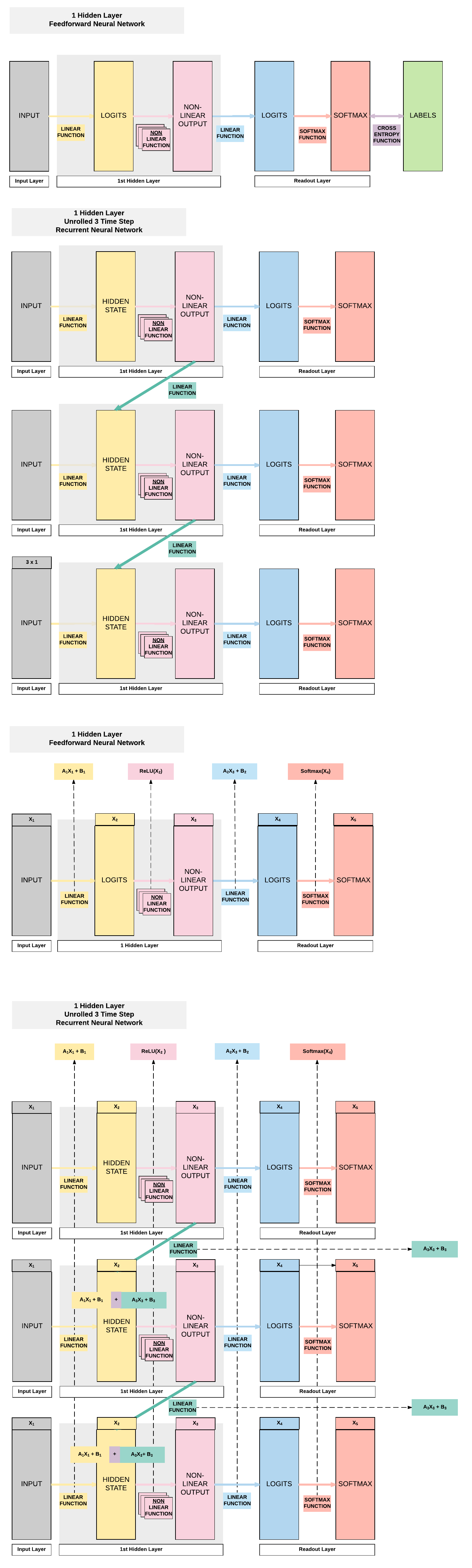
Feedforward Neural Networks Transition to 1 Layer Recurrent Neural Networks (RNN)

• RNN is essentially an FNN but with a hidden layer (non-linear output) that passes on information to the next FNN
• Compared to an FNN, we've one additional set of weight and bias that allows information to flow from one FNN to another FNN sequentially that allows time-dependency.
• The diagram below shows the only difference between an FNN and a RNN.

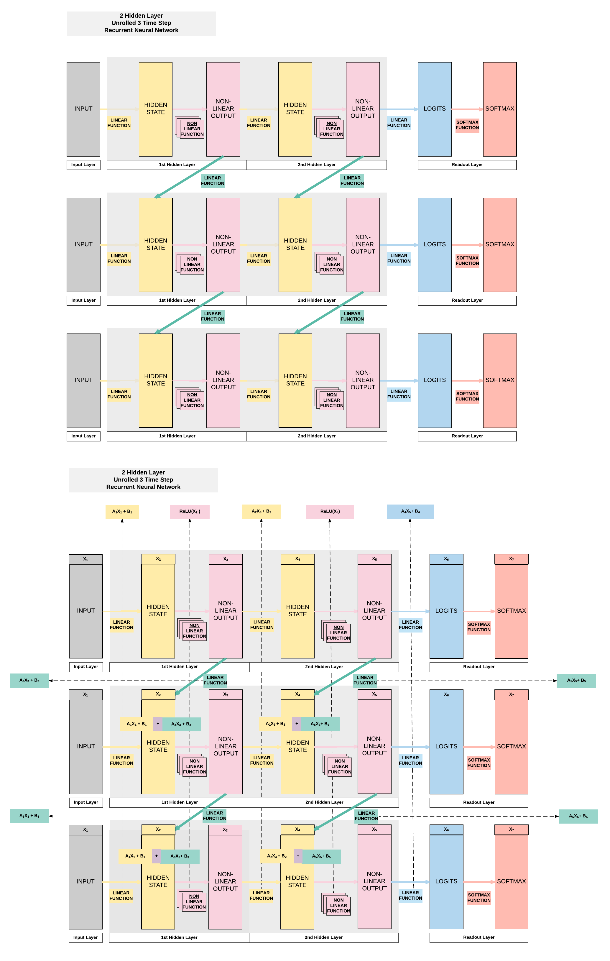
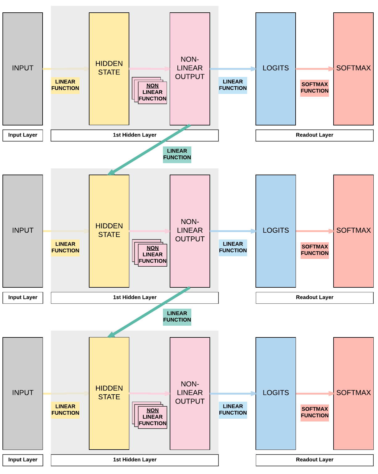
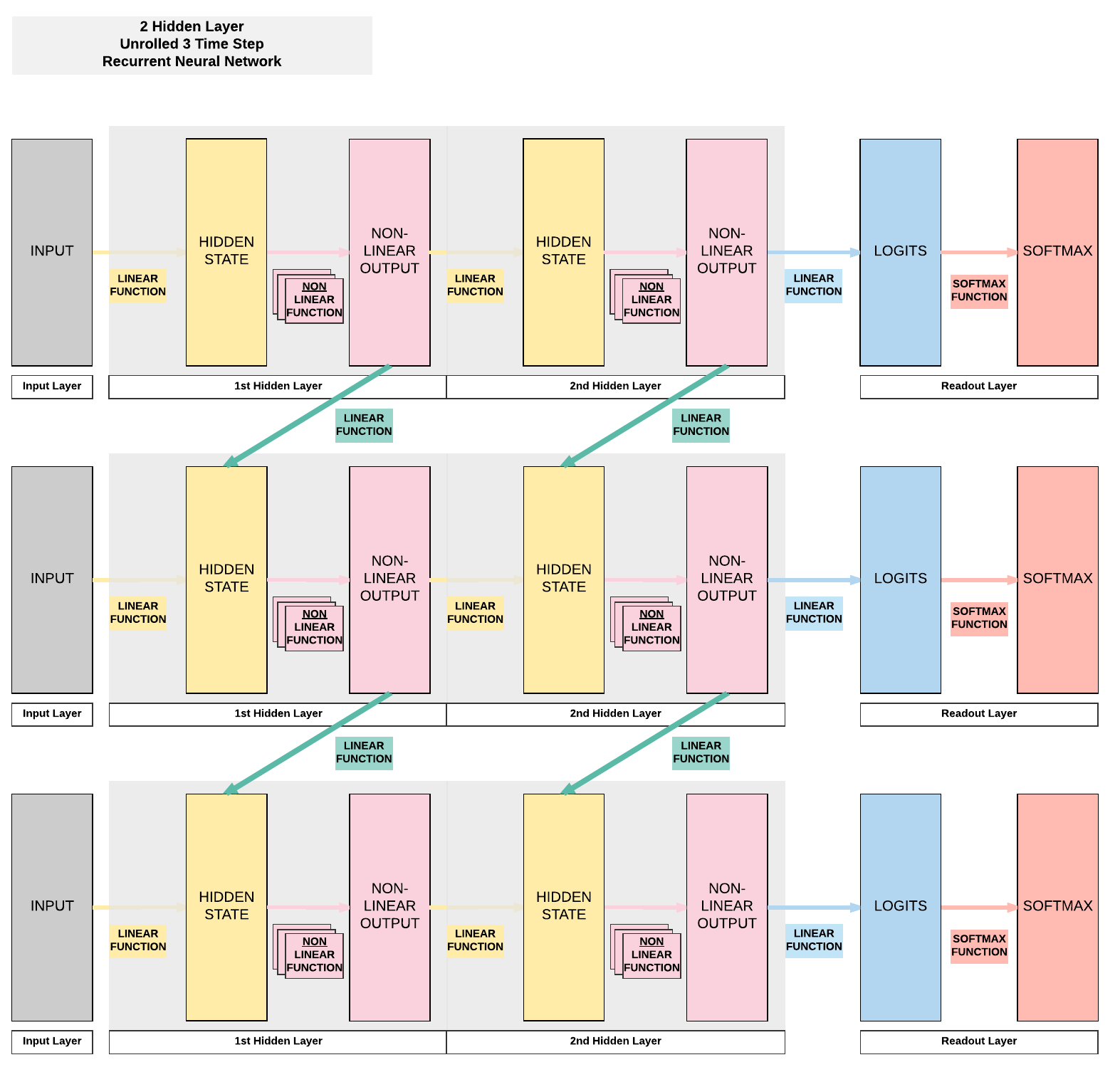
2 Layer RNN Breakdown

Building a Recurrent Neural Network with PyTorch

Model A: 1 Hidden Layer (ReLU)

• Unroll 28 time steps
  • Each step input size: 28 x 1
  • Total per unroll: 28 x 28
    • Feedforward Neural Network input size: 28 x 28
• 1 Hidden layer
• ReLU Activation Function

Steps

• Step 1: Load Dataset
• Step 2: Make Dataset Iterable
• Step 3: Create Model Class
• Step 4: Instantiate Model Class
• Step 5: Instantiate Loss Class
• Step 6: Instantiate Optimizer Class
• Step 7: Train Model

Step 1: Loading MNIST Train Dataset

Images from 1 to 9

Looking into the MNIST Dataset

import torch
import torch.nn as nn
import torchvision.transforms as transforms
import torchvision.datasets as dsets

train_dataset = dsets.MNIST(root='./data', 
                            train=True, 
                            transform=transforms.ToTensor(),
                            download=True)

test_dataset = dsets.MNIST(root='./data', 
                           train=False, 
                           transform=transforms.ToTensor())

We would have 60k training images of size 28 x 28 pixels.

print(train_dataset.train_data.size())

print(train_dataset.train_labels.size())

Here we would have 10k testing images of the same size, 28 x 28 pixels.

print(test_dataset.test_data.size())

print(test_dataset.test_labels.size())

torch.Size([60000, 28, 28])

torch.Size([60000])

torch.Size([10000, 28, 28])

torch.Size([10000])

Step 2: Make Dataset Iterable

Creating iterable objects to loop through subsequently

batch_size = 100
n_iters = 3000
num_epochs = n_iters / (len(train_dataset) / batch_size)
num_epochs = int(num_epochs)

train_loader = torch.utils.data.DataLoader(dataset=train_dataset, 
                                           batch_size=batch_size, 
                                           shuffle=True)

test_loader = torch.utils.data.DataLoader(dataset=test_dataset, 
                                          batch_size=batch_size, 
                                          shuffle=False)

Step 3: Create Model Class

1 Layer RNN

class RNNModel(nn.Module):
    def __init__(self, input_dim, hidden_dim, layer_dim, output_dim):
        super(RNNModel, self).__init__()
        # Hidden dimensions
        self.hidden_dim = hidden_dim

        # Number of hidden layers
        self.layer_dim = layer_dim

        # Building your RNN
        # batch_first=True causes input/output tensors to be of shape
        # (batch_dim, seq_dim, input_dim)
        # batch_dim = number of samples per batch
        self.rnn = nn.RNN(input_dim, hidden_dim, layer_dim, batch_first=True, nonlinearity='relu')

        # Readout layer
        self.fc = nn.Linear(hidden_dim, output_dim)

    def forward(self, x):
        # Initialize hidden state with zeros
        # (layer_dim, batch_size, hidden_dim)
        h0 = torch.zeros(self.layer_dim, x.size(0), self.hidden_dim).requires_grad_()

        # We need to detach the hidden state to prevent exploding/vanishing gradients
        # This is part of truncated backpropagation through time (BPTT)
        out, hn = self.rnn(x, h0.detach())

        # Index hidden state of last time step
        # out.size() --> 100, 28, 10
        # out[:, -1, :] --> 100, 10 --> just want last time step hidden states! 
        out = self.fc(out[:, -1, :]) 
        # out.size() --> 100, 10
        return out

Step 4: Instantiate Model Class

• 28 time steps
  • Each time step: input dimension = 28
• 1 hidden layer
• MNIST 1-9 digits \(\rightarrow\) output dimension = 10

Instantiate model class and assign to an object

input_dim = 28
hidden_dim = 100
layer_dim = 1
output_dim = 10

model = RNNModel(input_dim, hidden_dim, layer_dim, output_dim)

Step 5: Instantiate Loss Class

• Recurrent Neural Network: Cross Entropy Loss
  • Convolutional Neural Network: Cross Entropy Loss
  • Feedforward Neural Network: Cross Entropy Loss
  • Logistic Regression: Cross Entropy Loss
  • Linear Regression: MSE

Cross Entropy Loss for Classification Task

criterion = nn.CrossEntropyLoss()

Cross Entropy vs MSE

Take note that there are cases where RNN, CNN and FNN use MSE as a loss function.

We use cross entropy for classification tasks (predicting 0-9 digits in MNIST for example).

And we use MSE for regression tasks (predicting temperatures in every December in San Francisco for example).

Step 6: Instantiate Optimizer Class

• Simplified equation
  • \(\theta = \theta - \eta \cdot \nabla_\theta\)
    • \(\theta\): parameters (our tensors with gradient accumulation abilities)
    • \(\eta\): learning rate (how fast we want to learn)
    • \(\nabla_\theta\): gradients of loss with respect to the model's parameters
• Even simplier equation
  • parameters = parameters - learning_rate * parameters_gradients
  • At every iteration, we update our model's parameters

learning_rate = 0.01

optimizer = torch.optim.SGD(model.parameters(), lr=learning_rate)  

Parameters In-Depth

• Input to Hidden Layer Affine Function
  • A1, B1
• Hidden Layer to Output Affine Function
  • A2, B2
• Hidden Layer to Hidden Layer Affine Function
  • A3, B3

Total groups of parameters

We should have 6 groups as shown above.

len(list(model.parameters()))

6

Input to Hidden Weight

Remember we defined our hidden layer to have a size of 100. Because our input is a size of 28 at each time step, this gives rise to a weight matrix of 100 x 28.

# Input --> Hidden (A1)
list(model.parameters())[0].size()

torch.Size([100, 28])

Input to Hidden Bias

# Input --> Hidden BIAS (B1)
list(model.parameters())[2].size()

torch.Size([100])

Hidden to Hidden

# Hidden --> Hidden (A3)
list(model.parameters())[1].size()

torch.Size([100, 100])

Hidden to Hidden Bias

# Hidden --> Hidden BIAS(B3)
list(model.parameters())[3].size()

torch.Size([100])

Hidden to Output

# Hidden --> Output (A2)
list(model.parameters())[4].size()

torch.Size([10, 100])

Hidden to Output Bias

# Hidden --> Output BIAS (B2)
list(model.parameters())[5].size()

torch.Size([10])

Step 7: Train Model

• Process
  1. Convert inputs/labels to tensors with gradient accumulation abilities
     • RNN Input: (1, 28)
     • CNN Input: (1, 28, 28)
     • FNN Input: (1, 28*28)
  2. Clear gradient buffets
  3. Get output given inputs
  4. Get loss
  5. Get gradients w.r.t. parameters
  6. Update parameters using gradients
     • parameters = parameters - learning_rate * parameters_gradients
  7. REPEAT

Same 7 step process for training models

# Number of steps to unroll
seq_dim = 28  

iter = 0
for epoch in range(num_epochs):
    for i, (images, labels) in enumerate(train_loader):
        model.train()
        # Load images as tensors with gradient accumulation abilities
        images = images.view(-1, seq_dim, input_dim).requires_grad_()

        # Clear gradients w.r.t. parameters
        optimizer.zero_grad()

        # Forward pass to get output/logits
        # outputs.size() --> 100, 10
        outputs = model(images)

        # Calculate Loss: softmax --> cross entropy loss
        loss = criterion(outputs, labels)

        # Getting gradients w.r.t. parameters
        loss.backward()

        # Updating parameters
        optimizer.step()

        iter += 1

        if iter % 500 == 0:
            model.eval()
            # Calculate Accuracy         
            correct = 0
            total = 0
            # Iterate through test dataset
            for images, labels in test_loader:
                # Load images to a Torch tensors with gradient accumulation abilities
                images = images.view(-1, seq_dim, input_dim)

                # Forward pass only to get logits/output
                outputs = model(images)

                # Get predictions from the maximum value
                _, predicted = torch.max(outputs.data, 1)

                # Total number of labels
                total += labels.size(0)

                # Total correct predictions
                correct += (predicted == labels).sum()

            accuracy = 100 * correct / total

            # Print Loss
            print('Iteration: {}. Loss: {}. Accuracy: {}'.format(iter, loss.item(), accuracy))

Iteration: 500. Loss: 2.301494836807251. Accuracy: 12
Iteration: 1000. Loss: 2.2986037731170654. Accuracy: 14
Iteration: 1500. Loss: 2.278566598892212. Accuracy: 18
Iteration: 2000. Loss: 2.169614315032959. Accuracy: 21
Iteration: 2500. Loss: 1.1662731170654297. Accuracy: 51
Iteration: 3000. Loss: 0.9290509223937988. Accuracy: 71

Model B: 2 Hidden Layer (ReLU)

• Unroll 28 time steps
  • Each step input size: 28 x 1
  • Total per unroll: 28 x 28
    • Feedforward Neural Network inpt size: 28 x 28
• 2 Hidden layer
• ReLU Activation Function

Steps

• Step 1: Load Dataset
• Step 2: Make Dataset Iterable
• Step 3: Create Model Class
• Step 4: Instantiate Model Class
• Step 5: Instantiate Loss Class
• Step 6: Instantiate Optimizer Class
• Step 7: Train Model

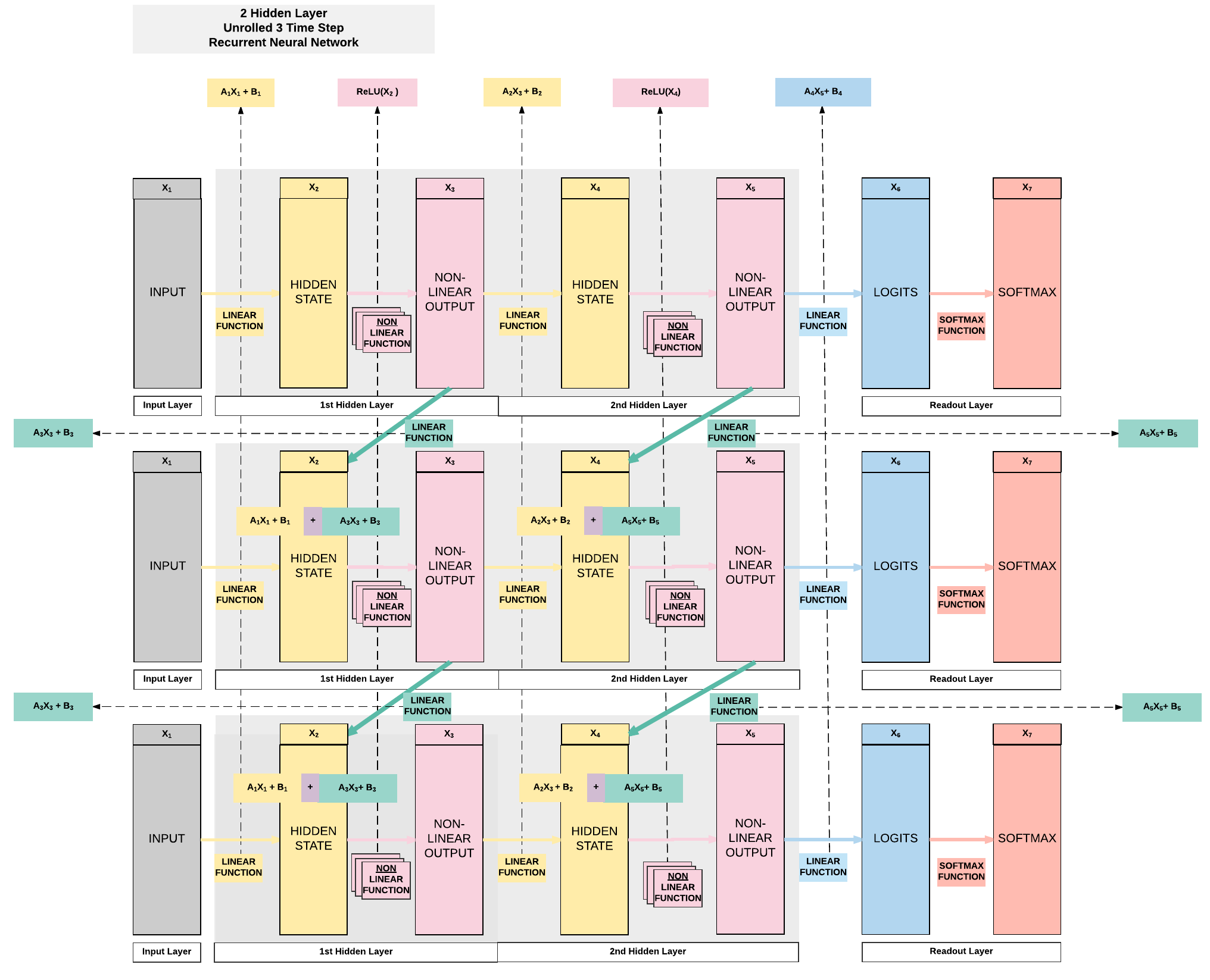
2 Hidden Layer + ReLU

import torch
import torch.nn as nn
import torchvision.transforms as transforms
import torchvision.datasets as dsets

'''
STEP 1: LOADING DATASET
'''
train_dataset = dsets.MNIST(root='./data', 
                            train=True, 
                            transform=transforms.ToTensor(),
                            download=True)

test_dataset = dsets.MNIST(root='./data', 
                           train=False, 
                           transform=transforms.ToTensor())

'''
STEP 2: MAKING DATASET ITERABLE
'''

batch_size = 100
n_iters = 3000
num_epochs = n_iters / (len(train_dataset) / batch_size)
num_epochs = int(num_epochs)

train_loader = torch.utils.data.DataLoader(dataset=train_dataset, 
                                           batch_size=batch_size, 
                                           shuffle=True)

test_loader = torch.utils.data.DataLoader(dataset=test_dataset, 
                                          batch_size=batch_size, 
                                          shuffle=False)

'''
STEP 3: CREATE MODEL CLASS
'''

class RNNModel(nn.Module):
    def __init__(self, input_dim, hidden_dim, layer_dim, output_dim):
        super(RNNModel, self).__init__()
        # Hidden dimensions
        self.hidden_dim = hidden_dim

        # Number of hidden layers
        self.layer_dim = layer_dim

        # Building your RNN
        # batch_first=True causes input/output tensors to be of shape
        # (batch_dim, seq_dim, feature_dim)
        self.rnn = nn.RNN(input_dim, hidden_dim, layer_dim, batch_first=True, nonlinearity='relu')

        # Readout layer
        self.fc = nn.Linear(hidden_dim, output_dim)

    def forward(self, x):
        # Initialize hidden state with zeros
        h0 = torch.zeros(self.layer_dim, x.size(0), self.hidden_dim).requires_grad_()

        # We need to detach the hidden state to prevent exploding/vanishing gradients
        # This is part of truncated backpropagation through time (BPTT)
        out, hn = self.rnn(x, h0.detach())

        # Index hidden state of last time step
        # out.size() --> 100, 28, 100
        # out[:, -1, :] --> 100, 100 --> just want last time step hidden states! 
        out = self.fc(out[:, -1, :]) 
        # out.size() --> 100, 10
        return out

'''
STEP 4: INSTANTIATE MODEL CLASS
'''
input_dim = 28
hidden_dim = 100
layer_dim = 2  # ONLY CHANGE IS HERE FROM ONE LAYER TO TWO LAYER
output_dim = 10

model = RNNModel(input_dim, hidden_dim, layer_dim, output_dim)

# JUST PRINTING MODEL & PARAMETERS 
print(model)
print(len(list(model.parameters())))
for i in range(len(list(model.parameters()))):
    print(list(model.parameters())[i].size())

'''
STEP 5: INSTANTIATE LOSS CLASS
'''
criterion = nn.CrossEntropyLoss()

'''
STEP 6: INSTANTIATE OPTIMIZER CLASS
'''
learning_rate = 0.01

optimizer = torch.optim.SGD(model.parameters(), lr=learning_rate)  

'''
STEP 7: TRAIN THE MODEL
'''

# Number of steps to unroll
seq_dim = 28  

iter = 0
for epoch in range(num_epochs):
    for i, (images, labels) in enumerate(train_loader):
        model.train()
        # Load images as tensors with gradient accumulation abilities
        images = images.view(-1, seq_dim, input_dim).requires_grad_()

        # Clear gradients w.r.t. parameters
        optimizer.zero_grad()

        # Forward pass to get output/logits
        # outputs.size() --> 100, 10
        outputs = model(images)

        # Calculate Loss: softmax --> cross entropy loss
        loss = criterion(outputs, labels)

        # Getting gradients w.r.t. parameters
        loss.backward()

        # Updating parameters
        optimizer.step()

        iter += 1

        if iter % 500 == 0:
            model.eval()
            # Calculate Accuracy         
            correct = 0
            total = 0
            # Iterate through test dataset
            for images, labels in test_loader:
                # Resize images
                images = images.view(-1, seq_dim, input_dim)

                # Forward pass only to get logits/output
                outputs = model(images)

                # Get predictions from the maximum value
                _, predicted = torch.max(outputs.data, 1)

                # Total number of labels
                total += labels.size(0)

                # Total correct predictions
                correct += (predicted == labels).sum()

            accuracy = 100 * correct / total

            # Print Loss
            print('Iteration: {}. Loss: {}. Accuracy: {}'.format(iter, loss.item(), accuracy))

RNNModel(
  (rnn): RNN(28, 100, num_layers=2, batch_first=True)
  (fc): Linear(in_features=100, out_features=10, bias=True)
)

10

torch.Size([100, 28])
torch.Size([100, 100])
torch.Size([100])
torch.Size([100])
torch.Size([100, 100])
torch.Size([100, 100])
torch.Size([100])
torch.Size([100])
torch.Size([10, 100])
torch.Size([10])

Iteration: 500. Loss: 2.3019518852233887. Accuracy: 11
Iteration: 1000. Loss: 2.299217700958252. Accuracy: 11
Iteration: 1500. Loss: 2.279090166091919. Accuracy: 14
Iteration: 2000. Loss: 2.126953125. Accuracy: 25
Iteration: 2500. Loss: 1.356347680091858. Accuracy: 57
Iteration: 3000. Loss: 0.7377720475196838. Accuracy: 69

• 10 sets of parameters
• First hidden Layer
  • \(A_1 = [100, 28]\)
  • \(A_3 = [100, 100]\)
  • \(B_1 = [100]\)
  • \(B_3 = [100]\)
• Second hidden layer
  • \(A_2 = [100, 100]\)
  • \(A_5 = [100, 100]\)
  • \(B_2 = [100]\)
  • \(B_5 = [100]\)
• Readout layer
  • \(A_4 = [10, 100]\)
  • \(B_4 = [10]\)

Model C: 2 Hidden Layer

• Unroll 28 time steps
  • Each step input size: 28 x 1
  • Total per unroll: 28 x 28
    • Feedforward Neural Network inpt size: 28 x 28
• 2 Hidden layer
• Tanh Activation Function

Steps

• Step 1: Load Dataset
• Step 2: Make Dataset Iterable
• Step 3: Create Model Class
• Step 4: Instantiate Model Class
• Step 5: Instantiate Loss Class
• Step 6: Instantiate Optimizer Class
• Step 7: Train Model

!!! "2 Hidden + ReLU"

import torch
import torch.nn as nn
import torchvision.transforms as transforms
import torchvision.datasets as dsets

'''
STEP 1: LOADING DATASET
'''
train_dataset = dsets.MNIST(root='./data', 
                            train=True, 
                            transform=transforms.ToTensor(),
                            download=True)

test_dataset = dsets.MNIST(root='./data', 
                           train=False, 
                           transform=transforms.ToTensor())

'''
STEP 2: MAKING DATASET ITERABLE
'''

batch_size = 100
n_iters = 3000
num_epochs = n_iters / (len(train_dataset) / batch_size)
num_epochs = int(num_epochs)

train_loader = torch.utils.data.DataLoader(dataset=train_dataset, 
                                           batch_size=batch_size, 
                                           shuffle=True)

test_loader = torch.utils.data.DataLoader(dataset=test_dataset, 
                                          batch_size=batch_size, 
                                          shuffle=False)

'''
STEP 3: CREATE MODEL CLASS
'''

class RNNModel(nn.Module):
    def __init__(self, input_dim, hidden_dim, layer_dim, output_dim):
        super(RNNModel, self).__init__()
        # Hidden dimensions
        self.hidden_dim = hidden_dim

        # Number of hidden layers
        self.layer_dim = layer_dim

        # Building your RNN
        # batch_first=True causes input/output tensors to be of shape
        # (batch_dim, seq_dim, feature_dim)
        self.rnn = nn.RNN(input_dim, hidden_dim, layer_dim, batch_first=True, nonlinearity='tanh')

        # Readout layer
        self.fc = nn.Linear(hidden_dim, output_dim)

    def forward(self, x):
        # Initialize hidden state with zeros
        h0 = torch.zeros(self.layer_dim, x.size(0), self.hidden_dim).requires_grad_()

        # One time step
        # We need to detach the hidden state to prevent exploding/vanishing gradients
        # This is part of truncated backpropagation through time (BPTT)
        out, hn = self.rnn(x, h0.detach())

        # Index hidden state of last time step
        # out.size() --> 100, 28, 100
        # out[:, -1, :] --> 100, 100 --> just want last time step hidden states! 
        out = self.fc(out[:, -1, :]) 
        # out.size() --> 100, 10
        return out

'''
STEP 4: INSTANTIATE MODEL CLASS
'''
input_dim = 28
hidden_dim = 100
layer_dim = 2  # ONLY CHANGE IS HERE FROM ONE LAYER TO TWO LAYER
output_dim = 10

model = RNNModel(input_dim, hidden_dim, layer_dim, output_dim)

# JUST PRINTING MODEL & PARAMETERS 
print(model)
print(len(list(model.parameters())))
for i in range(len(list(model.parameters()))):
    print(list(model.parameters())[i].size())

'''
STEP 5: INSTANTIATE LOSS CLASS
'''
criterion = nn.CrossEntropyLoss()

'''
STEP 6: INSTANTIATE OPTIMIZER CLASS
'''
learning_rate = 0.1

optimizer = torch.optim.SGD(model.parameters(), lr=learning_rate)  

'''
STEP 7: TRAIN THE MODEL
'''

# Number of steps to unroll
seq_dim = 28  

iter = 0
for epoch in range(num_epochs):
    for i, (images, labels) in enumerate(train_loader):
        # Load images as tensors with gradient accumulation abilities
        images = images.view(-1, seq_dim, input_dim).requires_grad_()

        # Clear gradients w.r.t. parameters
        optimizer.zero_grad()

        # Forward pass to get output/logits
        # outputs.size() --> 100, 10
        outputs = model(images)

        # Calculate Loss: softmax --> cross entropy loss
        loss = criterion(outputs, labels)

        # Getting gradients w.r.t. parameters
        loss.backward()

        # Updating parameters
        optimizer.step()

        iter += 1

        if iter % 500 == 0:
            # Calculate Accuracy         
            correct = 0
            total = 0
            # Iterate through test dataset
            for images, labels in test_loader:
                # Resize images
                images = images.view(-1, seq_dim, input_dim)

                # Forward pass only to get logits/output
                outputs = model(images)

                # Get predictions from the maximum value
                _, predicted = torch.max(outputs.data, 1)

                # Total number of labels
                total += labels.size(0)

                # Total correct predictions
                correct += (predicted == labels).sum()

            accuracy = 100 * correct / total

            # Print Loss
            print('Iteration: {}. Loss: {}. Accuracy: {}'.format(iter, loss.item(), accuracy))

RNNModel(
  (rnn): RNN(28, 100, num_layers=2, batch_first=True)
  (fc): Linear(in_features=100, out_features=10, bias=True)
)

10

torch.Size([100, 28])
torch.Size([100, 100])
torch.Size([100])
torch.Size([100])
torch.Size([100, 100])
torch.Size([100, 100])
torch.Size([100])
torch.Size([100])
torch.Size([10, 100])
torch.Size([10])
Iteration: 500. Loss: 0.5943437218666077. Accuracy: 77
Iteration: 1000. Loss: 0.22048641741275787. Accuracy: 91
Iteration: 1500. Loss: 0.18479223549365997. Accuracy: 94
Iteration: 2000. Loss: 0.2723771929740906. Accuracy: 91
Iteration: 2500. Loss: 0.18817797303199768. Accuracy: 92
Iteration: 3000. Loss: 0.1685929149389267. Accuracy: 92

Summary of Results

Model A	Model B	Model C
ReLU	ReLU	Tanh
1 Hidden Layer	2 Hidden Layers	2 Hidden Layers
100 Hidden Units	100 Hidden Units	100 Hidden Units
92.48%	95.09%	95.54%

General Deep Learning Notes

• 2 ways to expand a recurrent neural network
  • More non-linear activation units (neurons)
  • More hidden layers
• Cons
  • Need a larger dataset
    • Curse of dimensionality
  • Does not necessarily mean higher accuracy

3. Building a Recurrent Neural Network with PyTorch (GPU)

Model C: 2 Hidden Layer (Tanh)

GPU: 2 things must be on GPU - model - tensors

Steps

• Step 1: Load Dataset
• Step 2: Make Dataset Iterable
• Step 3: Create Model Class
• Step 4: Instantiate Model Class
• Step 5: Instantiate Loss Class
• Step 6: Instantiate Optimizer Class
• Step 7: Train Model

2 Layer RNN + Tanh

import torch
import torch.nn as nn
import torchvision.transforms as transforms
import torchvision.datasets as dsets

'''
STEP 1: LOADING DATASET
'''
train_dataset = dsets.MNIST(root='./data', 
                            train=True, 
                            transform=transforms.ToTensor(),
                            download=True)

test_dataset = dsets.MNIST(root='./data', 
                           train=False, 
                           transform=transforms.ToTensor())

'''
STEP 2: MAKING DATASET ITERABLE
'''

batch_size = 100
n_iters = 3000
num_epochs = n_iters / (len(train_dataset) / batch_size)
num_epochs = int(num_epochs)

train_loader = torch.utils.data.DataLoader(dataset=train_dataset, 
                                           batch_size=batch_size, 
                                           shuffle=True)

test_loader = torch.utils.data.DataLoader(dataset=test_dataset, 
                                          batch_size=batch_size, 
                                          shuffle=False)

'''
STEP 3: CREATE MODEL CLASS
'''

class RNNModel(nn.Module):
    def __init__(self, input_dim, hidden_dim, layer_dim, output_dim):
        super(RNNModel, self).__init__()
        # Hidden dimensions
        self.hidden_dim = hidden_dim

        # Number of hidden layers
        self.layer_dim = layer_dim

        # Building your RNN
        # batch_first=True causes input/output tensors to be of shape
        # (batch_dim, seq_dim, feature_dim)
        self.rnn = nn.RNN(input_dim, hidden_dim, layer_dim, batch_first=True, nonlinearity='tanh')

        # Readout layer
        self.fc = nn.Linear(hidden_dim, output_dim)

    def forward(self, x):
        # Initialize hidden state with zeros
        #######################
        #  USE GPU FOR MODEL  #
        #######################
        h0 = torch.zeros(self.layer_dim, x.size(0), self.hidden_dim).to(device)

        # One time step
        # We need to detach the hidden state to prevent exploding/vanishing gradients
        # This is part of truncated backpropagation through time (BPTT)
        out, hn = self.rnn(x, h0.detach())

        # Index hidden state of last time step
        # out.size() --> 100, 28, 100
        # out[:, -1, :] --> 100, 100 --> just want last time step hidden states! 
        out = self.fc(out[:, -1, :]) 
        # out.size() --> 100, 10
        return out

'''
STEP 4: INSTANTIATE MODEL CLASS
'''
input_dim = 28
hidden_dim = 100
layer_dim = 2  # ONLY CHANGE IS HERE FROM ONE LAYER TO TWO LAYER
output_dim = 10

model = RNNModel(input_dim, hidden_dim, layer_dim, output_dim)

#######################
#  USE GPU FOR MODEL  #
#######################

device = torch.device("cuda:0" if torch.cuda.is_available() else "cpu")
model.to(device)


'''
STEP 5: INSTANTIATE LOSS CLASS
'''
criterion = nn.CrossEntropyLoss()

'''
STEP 6: INSTANTIATE OPTIMIZER CLASS
'''
learning_rate = 0.1

optimizer = torch.optim.SGD(model.parameters(), lr=learning_rate)  

'''
STEP 7: TRAIN THE MODEL
'''

# Number of steps to unroll
seq_dim = 28  

iter = 0
for epoch in range(num_epochs):
    for i, (images, labels) in enumerate(train_loader):
        # Load images as tensors with gradient accumulation abilities
        #######################
        #  USE GPU FOR MODEL  #
        #######################
        images = images.view(-1, seq_dim, input_dim).requires_grad_().to(device)
        labels = labels.to(device)

        # Clear gradients w.r.t. parameters
        optimizer.zero_grad()

        # Forward pass to get output/logits
        # outputs.size() --> 100, 10
        outputs = model(images)

        # Calculate Loss: softmax --> cross entropy loss
        loss = criterion(outputs, labels)

        # Getting gradients w.r.t. parameters
        loss.backward()

        # Updating parameters
        optimizer.step()

        iter += 1

        if iter % 500 == 0:
            # Calculate Accuracy         
            correct = 0
            total = 0
            # Iterate through test dataset
            for images, labels in test_loader:
                #######################
                #  USE GPU FOR MODEL  #
                #######################
                images = images.view(-1, seq_dim, input_dim).to(device)

                # Forward pass only to get logits/output
                outputs = model(images)

                # Get predictions from the maximum value
                _, predicted = torch.max(outputs.data, 1)

                # Total number of labels
                total += labels.size(0)

                # Total correct predictions
                #######################
                #  USE GPU FOR MODEL  #
                #######################
                if torch.cuda.is_available():
                    correct += (predicted.cpu() == labels.cpu()).sum()
                else:
                    correct += (predicted == labels).sum()

            accuracy = 100 * correct / total

            # Print Loss
            print('Iteration: {}. Loss: {}. Accuracy: {}'.format(iter, loss.item(), accuracy))

Iteration: 500. Loss: 0.5983774662017822. Accuracy: 81
Iteration: 1000. Loss: 0.2960105836391449. Accuracy: 86
Iteration: 1500. Loss: 0.19428101181983948. Accuracy: 93
Iteration: 2000. Loss: 0.11918395012617111. Accuracy: 95
Iteration: 2500. Loss: 0.11246936023235321. Accuracy: 95
Iteration: 3000. Loss: 0.15849310159683228. Accuracy: 95

Summary

We've learnt to...

Success

• Feedforward Neural Networks Transition to Recurrent Neural Networks
• RNN Models in PyTorch
  • Model A: 1 Hidden Layer RNN (ReLU)
  • Model B: 2 Hidden Layer RNN (ReLU)
  • Model C: 2 Hidden Layer RNN (Tanh)
• Models Variation in Code
  • Modifying only step 4
• Ways to Expand Model’s Capacity
  • More non-linear activation units (neurons)
  • More hidden layers
• Cons of Expanding Capacity
  • Need more data
  • Does not necessarily mean higher accuracy
• GPU Code
  • 2 things on GPU
    • model
    • tensors with gradient accumulation abilities
  • Modifying only Step 3, 4 and 7
• 7 Step Model Building Recap
  • Step 1: Load Dataset
  • Step 2: Make Dataset Iterable
  • Step 3: Create Model Class
  • Step 4: Instantiate Model Class
  • Step 5: Instantiate Loss Class
  • Step 6: Instantiate Optimizer Class
  • Step 7: Train Model
  • Step 7: Train Model

Citation

If you have found these useful in your research, presentations, school work, projects or workshops, feel free to cite using this DOI.

Comments