Logistic Regression from Scratch¶

This is an implementation of a simple logistic regression for binary class labels. We will be attempting to classify 2 flowers based on their petal width and height: setosa and versicolor.

Imports¶

%matplotlib inline
import matplotlib.pyplot as plt
import numpy as np

import torch
import torch.nn.functional as F

from sklearn import datasets
from sklearn import preprocessing
from sklearn.model_selection import train_test_split
from collections import Counter

Preparing a custom 2-class IRIS dataset¶

Load Data¶

# Instantiate dataset class and assign to object
iris = datasets.load_iris()

# Load features and target
# Take only 2 classes, and 2 features (sepal length/width)
X = iris.data[:-50, :2]
# For teaching the math rather than preprocessing techniques,
# we'll be using this simple scaling method. However, you must
# be cautious to scale your training/testing sets subsequently.
X = preprocessing.scale(X)
y = iris.target[:-50]

Print Data Details¶

# 50 of each iris flower
print(Counter(y))

# Type of flower
print(list(iris.target_names[:-1]))

# Shape of features
print(X.shape)

Counter({0: 50, 1: 50})
['setosa', 'versicolor']
(100, 2)

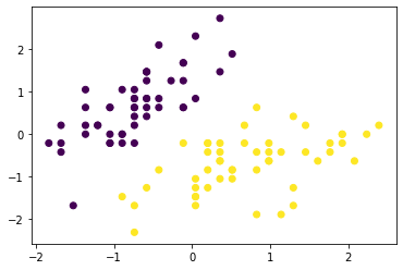
Scatterplot 2 Classes¶

plt.scatter(X[:, 0], X[:, 1], c=y);

png

Train/Test Split¶

X_train, X_test, y_train, y_test = train_test_split(X, y, test_size=0.2)
print(f'X train size: {X_train.shape}')
print(f'X test size: {X_test.shape}')
print(f'y train size: {y_train.shape}')
print(f'y test size: {y_test.shape}')

# Distribution of both classes are roughly equal using train_test_split function
print(Counter(y_train))

X train size: (80, 2)
X test size: (20, 2)
y train size: (80,)
y test size: (20,)
Counter({0: 41, 1: 39})

Math¶

1. Forwardpropagation¶

Get our logits and probabilities
Affine function/transformation: \(z = \theta x + b\)
Sigmoid/logistic function: \(\hat y = \frac{1}{1 + e^{-z}}\)

2. Backwardpropagation¶

Calculate gradients / partial derivatives w.r.t. weights and bias
Loss: \(L = ylog(\hat y) + (1-y) log (1 - \hat y)\)
Partial derivative of loss w.r.t weights: \(\frac{\delta L}{\delta w} =\frac{\delta L}{\delta z} \frac{\delta z}{\delta w} = (\hat y - y)(x^T)\)
Partial derivative of loss w.r.t. bias: \(\frac{\delta L}{\delta b} = \frac{\delta L}{\delta z} \frac{\delta z}{\delta b} = (\hat y - y)(1)\)
- \(\frac{\delta L}{\delta z} = \hat y - y\)
- \(\frac{\delta z}{\delta w} = x\)
- \(\frac{\delta z}{\delta b} = 1\)

2a. Loss function clarification¶

Actually, why is our loss equation \(L = ylog(\hat y) + (1-y) log (1 - \hat y)\)?
- We have given the intuition in the Logistic Regression tutorial on why it works.
- Here we will cover the derivation which essentially is merely maximizing the log likelihood of the parameters (maximizing the probability of our predicted output given our input and parameters
- Given:
  - \(\hat y = \frac{1}{1 + e^{-z}}\).
- Then:
  - \(P(y=1 \mid x;\theta) = \hat y\)
  - \(P(y=0 \mid x;\theta) = 1 - \hat y\)
- Simplified further:
  - \(p(y \mid x; \theta) = (\hat y)^y(1 - \hat y)^{1-y}\)
- Given m training samples, the likelihood of the parameters is simply the product of probabilities:
  - \(L(\theta) = \displaystyle \prod_{i=1}^{m} p(y^i \mid x^i; \theta)\)
  - \(L(\theta) = \displaystyle \prod_{i=1}^{m} (\hat y^{i})^{y^i}(1 - \hat y^{i})^{1-y^{i}}\)
  - Essentially, we want to maximize the probability of our ouput given our input and parameters
- But it's easier to maximize the log likelihood, so we take the natural logarithm.
  - \(L(\theta) = \displaystyle \sum_{i=1}^{m} y^{i}log (\hat y^{i}) + (1 - y^{i})log(1 - \hat y^{i})\)
- Why is is easier to maximize the log likelihood?
  - The natural logarithm is a function that monotonically increases.
  - This allows us to find the "max" of the log likelihood easier compared to a non-monotonically increasing function (like a wave up and down).

3. Gradient descent: updating weights¶

\(w = w - \alpha (\hat y - y)(x^T)\)
\(b = b - \alpha (\hat y - y).1\)

Training from Scratch¶

learning_rate = 0.1
num_features = X.shape[1]
weights = torch.zeros(num_features, 1, dtype=torch.float32)
bias = torch.zeros(1, dtype=torch.float32)

X_train = torch.from_numpy(X_train).type(torch.float32)
y_train = torch.from_numpy(y_train).type(torch.float32)

for epoch in range(num_epochs):        
    # 1. Forwardpropagation:
    # 1a. Affine Transformation: z = \theta x + b
    z = torch.add(torch.mm(X_train, weights), bias)
    # 2a. Sigmoid/Logistic Function: y_hat = 1 / (1 + e^{-z})
    y_hat = 1. / (1. + torch.exp(-z))

    # Backpropagation:
    # 1. Calculate binary cross entropy 
    l = torch.mm(-y_train.view(1, -1), torch.log(y_hat)) - torch.mm((1 - y_train).view(1, -1), torch.log(1 - y_hat))

    # 2. Calculate dl/dz
    dl_dz = y_train - y_hat.view(-1)

    # 2. Calculate partial derivative of cost w.r.t weights (gradients)
    # dl_dw = dl_dz dz_dw = (y_hat - y)(x^T)
    grad = torch.mm(X_train.transpose(0, 1), dl_dz.view(-1, 1))

    # Gradient descent:
    # update our weights and bias with our gradients
    weights += learning_rate * grad
    bias += learning_rate * torch.sum(dl_dz)

    # Accuracy
    total = y_hat.shape[0]
    predicted = (y_hat > 0.5).float().squeeze()
    correct = (predicted == y_train).sum()
    acc = 100 * correct / total 

    # Print accuracy and cost
    print(f'Epoch: {epoch} | Accuracy: {acc.item() :.4f} | Cost: {l.item() :.4f}')

print(f'Weights \n {weights.data}')
print(f'Bias \n {bias.data}')

X train size: (80, 2)
X test size: (20, 2)
y train size: (80,)
y test size: (20,)
Counter({1: 41, 0: 39})
Epoch: 0 | Accuracy: 48.0000 | Cost: 55.4518
Epoch: 1 | Accuracy: 100.0000 | Cost: 5.6060
Epoch: 2 | Accuracy: 100.0000 | Cost: 5.0319
Epoch: 3 | Accuracy: 100.0000 | Cost: 4.6001
Epoch: 4 | Accuracy: 100.0000 | Cost: 4.2595
Epoch: 5 | Accuracy: 100.0000 | Cost: 3.9819
Epoch: 6 | Accuracy: 100.0000 | Cost: 3.7498
Epoch: 7 | Accuracy: 100.0000 | Cost: 3.5521
Epoch: 8 | Accuracy: 100.0000 | Cost: 3.3810
Epoch: 9 | Accuracy: 100.0000 | Cost: 3.2310
Epoch: 10 | Accuracy: 100.0000 | Cost: 3.0981
Epoch: 11 | Accuracy: 100.0000 | Cost: 2.9794
Epoch: 12 | Accuracy: 100.0000 | Cost: 2.8724
Epoch: 13 | Accuracy: 100.0000 | Cost: 2.7754
Epoch: 14 | Accuracy: 100.0000 | Cost: 2.6869
Epoch: 15 | Accuracy: 100.0000 | Cost: 2.6057
Epoch: 16 | Accuracy: 100.0000 | Cost: 2.5308
Epoch: 17 | Accuracy: 100.0000 | Cost: 2.4616
Epoch: 18 | Accuracy: 100.0000 | Cost: 2.3973
Epoch: 19 | Accuracy: 100.0000 | Cost: 2.3374
Weights 
 tensor([[ 4.9453],
        [-3.6849]])
Bias 
 tensor([0.5570])

Inference¶

# Port to tensors
X_test = torch.from_numpy(X_test).type(torch.float32)
y_test = torch.from_numpy(y_test).type(torch.float32)

# 1. Forwardpropagation:
# 1a. Affine Transformation: z = ax + b
z = torch.add(torch.mm(X_test, weights), bias)
# 2a. Sigmoid/Logistic Function: y_hat = 1 / (1 + e^{-z})
y_hat = 1. / (1. + torch.exp(-z))

total = y_test.shape[0]
predicted = (y_hat > 0.5).float().squeeze()
correct = (predicted == y_test).sum()
acc = 100 * correct / total 

# Print accuracy
print(f'Validation Accuracy: {acc.item() :.4f}')

Validation Accuracy: 100.0000

Logistic Regression from Scratch¶

Imports¶

Preparing a custom 2-class IRIS dataset¶

Load Data¶

Print Data Details¶

Scatterplot 2 Classes¶

Train/Test Split¶

Math¶

1. Forwardpropagation¶

2. Backwardpropagation¶

2a. Loss function clarification¶

3. Gradient descent: updating weights¶

Training from Scratch¶

Inference¶

Comments