Long Short-Term Memory (LSTM) network with PyTorch
Run Jupyter Notebook
You can run the code for this section in this jupyter notebook link.
About LSTMs: Special RNN
- Capable of learning long-term dependencies
- LSTM = RNN on super juice
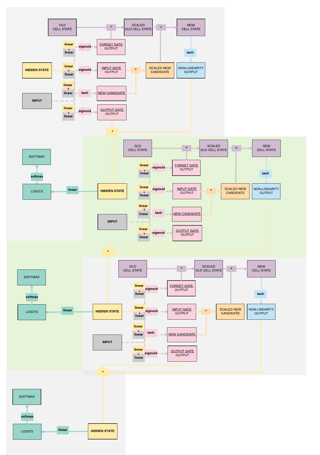
RNN Transition to LSTM
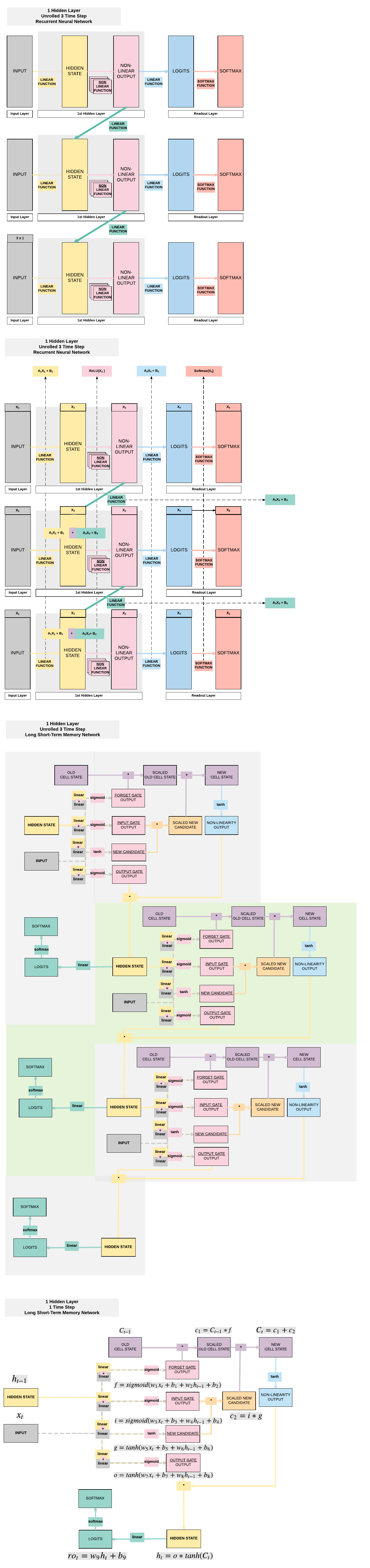
Building an LSTM with PyTorch
Model A: 1 Hidden Layer
- Unroll 28 time steps
- Each step input size: 28 x 1
- Total per unroll: 28 x 28
- Feedforward Neural Network input size: 28 x 28
- 1 Hidden layer
Steps
- Step 1: Load Dataset
- Step 2: Make Dataset Iterable
- Step 3: Create Model Class
- Step 4: Instantiate Model Class
- Step 5: Instantiate Loss Class
- Step 6: Instantiate Optimizer Class
- Step 7: Train Model
Step 1: Loading MNIST Train Dataset
Images from 1 to 9
The usual loading of our MNIST dataset
As usual, we've 60k training images and 10k testing images.
Subsequently, we'll have 3 groups: training, validation and testing for a more robust evaluation of algorithms.
import torch
import torch.nn as nn
import torchvision.transforms as transforms
import torchvision.datasets as dsets
train_dataset = dsets.MNIST(root='./data',
                            train=True,
                            transform=transforms.ToTensor(),
                            download=True)

test_dataset = dsets.MNIST(root='./data',
                           train=False,
                           transform=transforms.ToTensor())
print(train_dataset.train_data.size())
print(train_dataset.train_labels.size())
print(test_dataset.test_data.size())


```python
print(test_dataset.test_labels.size())
torch.Size([60000, 28, 28])
torch.Size([60000])

torch.Size([10000, 28, 28])
torch.Size([10000])
Step 2: Make Dataset Iterable
Creating an iterable object for our dataset
batch_size = 100
n_iters = 3000
num_epochs = n_iters / (len(train_dataset) / batch_size)
num_epochs = int(num_epochs)

train_loader = torch.utils.data.DataLoader(dataset=train_dataset,
                                           batch_size=batch_size,
                                           shuffle=True)

test_loader = torch.utils.data.DataLoader(dataset=test_dataset,
                                          batch_size=batch_size,
                                          shuffle=False)
Step 3: Create Model Class
Creating an LSTM model class
It is very similar to RNN in terms of the shape of our input of batch_dim x seq_dim x feature_dim.
The only change is that we have our cell state on top of our hidden state. PyTorch's LSTM module handles all the other weights for our other gates.
class LSTMModel(nn.Module):
    def __init__(self, input_dim, hidden_dim, layer_dim, output_dim):
        super(LSTMModel, self).__init__()
        # Hidden dimensions
        self.hidden_dim = hidden_dim

        # Number of hidden layers
        self.layer_dim = layer_dim

        # Building your LSTM
        # batch_first=True causes input/output tensors to be of shape
        # (batch_dim, seq_dim, feature_dim)
        self.lstm = nn.LSTM(input_dim, hidden_dim, layer_dim, batch_first=True)

        # Readout layer
        self.fc = nn.Linear(hidden_dim, output_dim)

    def forward(self, x):
        # Initialize hidden state with zeros
        h0 = torch.zeros(self.layer_dim, x.size(0), self.hidden_dim).requires_grad_()

        # Initialize cell state
        c0 = torch.zeros(self.layer_dim, x.size(0), self.hidden_dim).requires_grad_()

        # 28 time steps
        # We need to detach as we are doing truncated backpropagation through time (BPTT)
        # If we don't, we'll backprop all the way to the start even after going through another batch
        out, (hn, cn) = self.lstm(x, (h0.detach(), c0.detach()))

        # Index hidden state of last time step
        # out.size() --> 100, 28, 100
        # out[:, -1, :] --> 100, 100 --> just want last time step hidden states!
        out = self.fc(out[:, -1, :])
        # out.size() --> 100, 10
        return out
Step 4: Instantiate Model Class
- 28 time steps
- Each time step: input dimension = 28
- 1 hidden layer
- MNIST 1-9 digits \(\rightarrow\) output dimension = 10
Instantiate our LSTM model
input_dim = 28
hidden_dim = 100
layer_dim = 1
output_dim = 10
model = LSTMModel(input_dim, hidden_dim, layer_dim, output_dim)
Step 5: Instantiate Loss Class
- Long Short-Term Memory Neural Network: Cross Entropy Loss
- Recurrent Neural Network: Cross Entropy Loss
- Convolutional Neural Network: Cross Entropy Loss
- Feedforward Neural Network: Cross Entropy Loss
- Logistic Regression: Cross Entropy Loss
- Linear Regression: MSE
Cross Entry Loss Function
Because we are doing a classification problem we'll be using a Cross Entropy function. If we were to do a regression problem, then we would typically use a MSE function.
criterion = nn.CrossEntropyLoss()
Step 6: Instantiate Optimizer Class
- Simplified equation
- \(\theta = \theta - \eta \cdot \nabla_\theta\)
- \(\theta\): parameters (our variables)
- \(\eta\): learning rate (how fast we want to learn)
- \(\nabla_\theta\): parameters' gradients
- \(\theta = \theta - \eta \cdot \nabla_\theta\)
- Even simplier equation
parameters = parameters - learning_rate * parameters_gradients- At every iteration, we update our model's parameters
Mini-batch Stochastic Gradient Descent
learning_rate = 0.1

optimizer = torch.optim.SGD(model.parameters(), lr=learning_rate)
Parameters In-Depth
1 Layer LSTM Groups of Parameters
We will have 6 groups of parameters here comprising weights and biases from: - Input to Hidden Layer Affine Function - Hidden Layer to Output Affine Function - Hidden Layer to Hidden Layer Affine Function
Notice how this is exactly the same number of groups of parameters as our RNN? But the sizes of these groups will be larger for an LSTM due to its gates.
len(list(model.parameters()))
6
In-depth Parameters Analysis
Comparing to RNN's parameters, we've the same number of groups but for LSTM we've 4x the number of parameters!
for i in range(len(list(model.parameters()))):
    print(list(model.parameters())[i].size())
torch.Size([400, 28])
torch.Size([400, 100])

torch.Size([400])
torch.Size([400])

torch.Size([10, 100])
torch.Size([10])
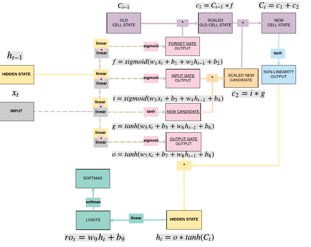
Parameters Breakdown
- This is the breakdown of the parameters associated with the respective affine functions
- Input \(\rightarrow\) Gates
- \([400, 28] \rightarrow w_1, w_3, w_5, w_7\)
- \([400] \rightarrow b_1, b_3, b_5, b_7\)
- Hidden State \(\rightarrow\) Gates
- \([400,100] \rightarrow w_2, w_4, w_6, w_8\)
- \([400] \rightarrow b_2, b_4, b_6, b_8\)
- Hidden State \(\rightarrow\) Output
- \([10, 100] \rightarrow w_9\)
- \([10] \rightarrow b_9\)
Step 7: Train Model
- Process
- Convert inputs/labels to variables
- LSTM Input: (1, 28)
- RNN Input: (1, 28)
- CNN Input: (1, 28, 28)
- FNN Input: (1, 28*28)
- Clear gradient buffets
- Get output given inputs
- Get loss
- Get gradients w.r.t. parameters
- Update parameters using gradients
parameters = parameters - learning_rate * parameters_gradients
- REPEAT
- Convert inputs/labels to variables
Training 1 Hidden Layer LSTM
# Number of steps to unroll
seq_dim = 28

iter = 0
for epoch in range(num_epochs):
    for i, (images, labels) in enumerate(train_loader):
        # Load images as a torch tensor with gradient accumulation abilities
        images = images.view(-1, seq_dim, input_dim).requires_grad_()

        # Clear gradients w.r.t. parameters
        optimizer.zero_grad()

        # Forward pass to get output/logits
        # outputs.size() --> 100, 10
        outputs = model(images)

        # Calculate Loss: softmax --> cross entropy loss
        loss = criterion(outputs, labels)

        # Getting gradients w.r.t. parameters
        loss.backward()

        # Updating parameters
        optimizer.step()

        iter += 1

        if iter % 500 == 0:
            # Calculate Accuracy
            correct = 0
            total = 0
            # Iterate through test dataset
            for images, labels in test_loader:
                # Resize images
                images = images.view(-1, seq_dim, input_dim)

                # Forward pass only to get logits/output
                outputs = model(images)

                # Get predictions from the maximum value
                _, predicted = torch.max(outputs.data, 1)

                # Total number of labels
                total += labels.size(0)

                # Total correct predictions
                correct += (predicted == labels).sum()

            accuracy = 100 * correct / total

            # Print Loss
            print('Iteration: {}. Loss: {}. Accuracy: {}'.format(iter, loss.item(), accuracy))
Iteration: 500. Loss: 0.8390830755233765. Accuracy: 72
Iteration: 1000. Loss: 0.46470555663108826. Accuracy: 85
Iteration: 1500. Loss: 0.31465113162994385. Accuracy: 91
Iteration: 2000. Loss: 0.19143860042095184. Accuracy: 94
Iteration: 2500. Loss: 0.16134005784988403. Accuracy: 95
Iteration: 3000. Loss: 0.255976140499115. Accuracy: 95
Model B: 2 Hidden Layer
- Unroll 28 time steps
- Each step input size: 28 x 1
- Total per unroll: 28 x 28
- Feedforward Neural Network inpt size: 28 x 28
- 2 Hidden layer
Steps
- Step 1: Load Dataset
- Step 2: Make Dataset Iterable
- Step 3: Create Model Class
- Step 4: Instantiate Model Class
- Step 5: Instantiate Loss Class
- Step 6: Instantiate Optimizer Class
- Step 7: Train Model
Train 2 Hidden Layer LSTM
import torch
import torch.nn as nn
import torchvision.transforms as transforms
import torchvision.datasets as dsets

'''
STEP 1: LOADING DATASET
'''
train_dataset = dsets.MNIST(root='./data',
                            train=True,
                            transform=transforms.ToTensor(),
                            download=True)

test_dataset = dsets.MNIST(root='./data',
                           train=False,
                           transform=transforms.ToTensor())

'''
STEP 2: MAKING DATASET ITERABLE
'''

batch_size = 100
n_iters = 3000
num_epochs = n_iters / (len(train_dataset) / batch_size)
num_epochs = int(num_epochs)

train_loader = torch.utils.data.DataLoader(dataset=train_dataset,
                                           batch_size=batch_size,
                                           shuffle=True)

test_loader = torch.utils.data.DataLoader(dataset=test_dataset,
                                          batch_size=batch_size,
                                          shuffle=False)

'''
STEP 3: CREATE MODEL CLASS
'''

class LSTMModel(nn.Module):
    def __init__(self, input_dim, hidden_dim, layer_dim, output_dim):
        super(LSTMModel, self).__init__()
        # Hidden dimensions
        self.hidden_dim = hidden_dim

        # Number of hidden layers
        self.layer_dim = layer_dim

        # Building your LSTM
        # batch_first=True causes input/output tensors to be of shape
        # (batch_dim, seq_dim, feature_dim)
        self.lstm = nn.LSTM(input_dim, hidden_dim, layer_dim, batch_first=True)

        # Readout layer
        self.fc = nn.Linear(hidden_dim, output_dim)

    def forward(self, x):
        # Initialize hidden state with zeros
        h0 = torch.zeros(self.layer_dim, x.size(0), self.hidden_dim).requires_grad_()

        # Initialize cell state
        c0 = torch.zeros(self.layer_dim, x.size(0), self.hidden_dim).requires_grad_()

        # One time step
        # We need to detach as we are doing truncated backpropagation through time (BPTT)
        # If we don't, we'll backprop all the way to the start even after going through another batch
        out, (hn, cn) = self.lstm(x, (h0.detach(), c0.detach()))

        # Index hidden state of last time step
        # out.size() --> 100, 28, 100
        # out[:, -1, :] --> 100, 100 --> just want last time step hidden states!
        out = self.fc(out[:, -1, :])
        # out.size() --> 100, 10
        return out

'''
STEP 4: INSTANTIATE MODEL CLASS
'''
input_dim = 28
hidden_dim = 100
layer_dim = 2  # ONLY CHANGE IS HERE FROM ONE LAYER TO TWO LAYER
output_dim = 10

model = LSTMModel(input_dim, hidden_dim, layer_dim, output_dim)

# JUST PRINTING MODEL & PARAMETERS
print(model)
print(len(list(model.parameters())))
for i in range(len(list(model.parameters()))):
    print(list(model.parameters())[i].size())

'''
STEP 5: INSTANTIATE LOSS CLASS
'''
criterion = nn.CrossEntropyLoss()

'''
STEP 6: INSTANTIATE OPTIMIZER CLASS
'''
learning_rate = 0.1

optimizer = torch.optim.SGD(model.parameters(), lr=learning_rate)

'''
STEP 7: TRAIN THE MODEL
'''

# Number of steps to unroll
seq_dim = 28

iter = 0
for epoch in range(num_epochs):
    for i, (images, labels) in enumerate(train_loader):
        # Load images as torch tensor with gradient accumulation abilities
        images = images.view(-1, seq_dim, input_dim).requires_grad_()

        # Clear gradients w.r.t. parameters
        optimizer.zero_grad()

        # Forward pass to get output/logits
        # outputs.size() --> 100, 10
        outputs = model(images)

        # Calculate Loss: softmax --> cross entropy loss
        loss = criterion(outputs, labels)

        # Getting gradients w.r.t. parameters
        loss.backward()

        # Updating parameters
        optimizer.step()

        iter += 1

        if iter % 500 == 0:
            # Calculate Accuracy
            correct = 0
            total = 0
            # Iterate through test dataset
            for images, labels in test_loader:
                # Resize image
                images = images.view(-1, seq_dim, input_dim)

                # Forward pass only to get logits/output
                outputs = model(images)

                # Get predictions from the maximum value
                _, predicted = torch.max(outputs.data, 1)

                # Total number of labels
                total += labels.size(0)

                # Total correct predictions
                correct += (predicted == labels).sum()

            accuracy = 100 * correct / total

            # Print Loss
            print('Iteration: {}. Loss: {}. Accuracy: {}'.format(iter, loss.item(), accuracy))
LSTMModel(
  (lstm): LSTM(28, 100, num_layers=2, batch_first=True)
  (fc): Linear(in_features=100, out_features=10, bias=True)
)

10

torch.Size([400, 28])
torch.Size([400, 100])
torch.Size([400])
torch.Size([400])
torch.Size([400, 100])
torch.Size([400, 100])
torch.Size([400])
torch.Size([400])
torch.Size([10, 100])
torch.Size([10])

Iteration: 500. Loss: 2.3074915409088135. Accuracy: 11
Iteration: 1000. Loss: 1.8854578733444214. Accuracy: 35
Iteration: 1500. Loss: 0.5317062139511108. Accuracy: 80
Iteration: 2000. Loss: 0.15290376543998718. Accuracy: 92
Iteration: 2500. Loss: 0.19500978291034698. Accuracy: 93
Iteration: 3000. Loss: 0.10683634132146835. Accuracy: 95
Parameters Breakdown (Layer 1)
- Input \(\rightarrow\) Gates
- \([400, 28]\)
- \([400]\)
- Hidden State \(\rightarrow\) Gates
- \([400,100]\)
- \([400]\)
Parameters Breakdown (Layer 2)
- Input \(\rightarrow\) Gates
- \([400, 100]\)
- \([400]\)
- Hidden State \(\rightarrow\) Gates
- \([400,100]\)
- \([400]\)
Parameters Breakdown (Readout Layer)
- Hidden State \(\rightarrow\) Output
- \([10, 100]\)
- \([10]\)
Model C: 3 Hidden Layer
- Unroll 28 time steps
- Each step input size: 28 x 1
- Total per unroll: 28 x 28
- Feedforward Neural Network inpt size: 28 x 28
- 3 Hidden layer
Steps
- Step 1: Load Dataset
- Step 2: Make Dataset Iterable
- Step 3: Create Model Class
- Step 4: Instantiate Model Class
- Step 5: Instantiate Loss Class
- Step 6: Instantiate Optimizer Class
- Step 7: Train Model
3 Hidden Layer LSTM
import torch
import torch.nn as nn
import torchvision.transforms as transforms
import torchvision.datasets as dsets

'''
STEP 1: LOADING DATASET
'''
train_dataset = dsets.MNIST(root='./data',
                            train=True,
                            transform=transforms.ToTensor(),
                            download=True)

test_dataset = dsets.MNIST(root='./data',
                           train=False,
                           transform=transforms.ToTensor())

'''
STEP 2: MAKING DATASET ITERABLE
'''

batch_size = 100
n_iters = 3000
num_epochs = n_iters / (len(train_dataset) / batch_size)
num_epochs = int(num_epochs)

train_loader = torch.utils.data.DataLoader(dataset=train_dataset,
                                           batch_size=batch_size,
                                           shuffle=True)

test_loader = torch.utils.data.DataLoader(dataset=test_dataset,
                                          batch_size=batch_size,
                                          shuffle=False)

'''
STEP 3: CREATE MODEL CLASS
'''

class LSTMModel(nn.Module):
    def __init__(self, input_dim, hidden_dim, layer_dim, output_dim):
        super(LSTMModel, self).__init__()
        # Hidden dimensions
        self.hidden_dim = hidden_dim

        # Number of hidden layers
        self.layer_dim = layer_dim

        # Building your LSTM
        # batch_first=True causes input/output tensors to be of shape
        # (batch_dim, seq_dim, feature_dim)
        self.lstm = nn.LSTM(input_dim, hidden_dim, layer_dim, batch_first=True)

        # Readout layer
        self.fc = nn.Linear(hidden_dim, output_dim)

    def forward(self, x):
        # Initialize hidden state with zeros
        h0 = torch.zeros(self.layer_dim, x.size(0), self.hidden_dim).requires_grad_()

        # Initialize cell state
        c0 = torch.zeros(self.layer_dim, x.size(0), self.hidden_dim).requires_grad_()

        # One time step
        # We need to detach as we are doing truncated backpropagation through time (BPTT)
        # If we don't, we'll backprop all the way to the start even after going through another batch
        out, (hn, cn) = self.lstm(x, (h0.detach(), c0.detach()))

        # Index hidden state of last time step
        # out.size() --> 100, 28, 100
        # out[:, -1, :] --> 100, 100 --> just want last time step hidden states!
        out = self.fc(out[:, -1, :])
        # out.size() --> 100, 10
        return out

'''
STEP 4: INSTANTIATE MODEL CLASS
'''
input_dim = 28
hidden_dim = 100
layer_dim = 3  # ONLY CHANGE IS HERE FROM ONE LAYER TO TWO LAYER
output_dim = 10

model = LSTMModel(input_dim, hidden_dim, layer_dim, output_dim)

# JUST PRINTING MODEL & PARAMETERS
print(model)
print(len(list(model.parameters())))
for i in range(len(list(model.parameters()))):
    print(list(model.parameters())[i].size())

'''
STEP 5: INSTANTIATE LOSS CLASS
'''
criterion = nn.CrossEntropyLoss()

'''
STEP 6: INSTANTIATE OPTIMIZER CLASS
'''
learning_rate = 0.1

optimizer = torch.optim.SGD(model.parameters(), lr=learning_rate)

'''
STEP 7: TRAIN THE MODEL
'''

# Number of steps to unroll
seq_dim = 28

iter = 0
for epoch in range(num_epochs):
    for i, (images, labels) in enumerate(train_loader):
        # Load images as Variable
        images = images.view(-1, seq_dim, input_dim).requires_grad_()

        # Clear gradients w.r.t. parameters
        optimizer.zero_grad()

        # Forward pass to get output/logits
        # outputs.size() --> 100, 10
        outputs = model(images)

        # Calculate Loss: softmax --> cross entropy loss
        loss = criterion(outputs, labels)

        # Getting gradients w.r.t. parameters
        loss.backward()

        # Updating parameters
        optimizer.step()

        iter += 1

        if iter % 500 == 0:
            # Calculate Accuracy
            correct = 0
            total = 0
            # Iterate through test dataset
            for images, labels in test_loader:
                # Load images to a Torch Variable
                images = images.view(-1, seq_dim, input_dim).requires_grad_()

                # Forward pass only to get logits/output
                outputs = model(images)

                # Get predictions from the maximum value
                _, predicted = torch.max(outputs.data, 1)

                # Total number of labels
                total += labels.size(0)

                # Total correct predictions
                correct += (predicted == labels).sum()

            accuracy = 100 * correct / total

            # Print Loss
            print('Iteration: {}. Loss: {}. Accuracy: {}'.format(iter, loss.item(), accuracy))
LSTMModel(
  (lstm): LSTM(28, 100, num_layers=3, batch_first=True)
  (fc): Linear(in_features=100, out_features=10, bias=True)
)

14

torch.Size([400, 28])
torch.Size([400, 100])
torch.Size([400])
torch.Size([400])
torch.Size([400, 100])
torch.Size([400, 100])
torch.Size([400])
torch.Size([400])
torch.Size([400, 100])
torch.Size([400, 100])
torch.Size([400])
torch.Size([400])
torch.Size([10, 100])
torch.Size([10])

Iteration: 500. Loss: 2.2927396297454834. Accuracy: 11
Iteration: 1000. Loss: 2.29740309715271. Accuracy: 11
Iteration: 1500. Loss: 2.1950502395629883. Accuracy: 20
Iteration: 2000. Loss: 1.0738657712936401. Accuracy: 59
Iteration: 2500. Loss: 0.5988132357597351. Accuracy: 79
Iteration: 3000. Loss: 0.4107239246368408. Accuracy: 88
Parameters Breakdown (Layer 1)
- Input \(\rightarrow\) Gates
- [400, 28]
- [400]
- Hidden State \(\rightarrow\) Gates
- [400,100]
- [400]
Parameters Breakdown (Layer 2)
- Input \(\rightarrow\) Gates
- [400, 100]
- [400]
- Hidden State \(\rightarrow\) Gates
- [400,100]
- [400]
Parameters Breakdown (Layer 3)
- Input \(\rightarrow\) Gates
- [400, 100]
- [400]
- Hidden State \(\rightarrow\) Gates
- [400,100]
- [400]
Parameters Breakdown (Readout Layer)
- Hidden State \(\rightarrow\) Output
- [10, 100]
- [10]
Comparison with RNN
| Model A RNN | Model B RNN | Model C RNN |
|---|---|---|
| ReLU | ReLU | Tanh |
| 1 Hidden Layer | 2 Hidden Layers | 3 Hidden Layers |
| 100 Hidden Units | 100 Hidden Units | 100 Hidden Units |
| 92.48% | 95.09% | 95.54% |
| Model A LSTM | Model B LSTM | Model C LSTM |
|---|---|---|
| 1 Hidden Layer | 2 Hidden Layers | 3 Hidden Layers |
| 100 Hidden Units | 100 Hidden Units | 100 Hidden Units |
| 96.05% | 95.24% | 91.22% |
Deep Learning Notes
- 2 ways to expand a recurrent neural network
- More hidden units
(o, i, f, g) gates
- More hidden layers
- More hidden units
- Cons
- Need a larger dataset
- Curse of dimensionality
- Does not necessarily mean higher accuracy
- Need a larger dataset
3. Building a Recurrent Neural Network with PyTorch (GPU)
Model A: 3 Hidden Layers
GPU: 2 things must be on GPU
- model
- tensors
Steps
- Step 1: Load Dataset
- Step 2: Make Dataset Iterable
- Step 3: Create Model Class
- Step 4: Instantiate Model Class
- Step 5: Instantiate Loss Class
- Step 6: Instantiate Optimizer Class
- Step 7: Train Model
3 Hidden Layer LSTM on GPU
import torch
import torch.nn as nn
import torchvision.transforms as transforms
import torchvision.datasets as dsets

'''
STEP 1: LOADING DATASET
'''
train_dataset = dsets.MNIST(root='./data',
                            train=True,
                            transform=transforms.ToTensor(),
                            download=True)

test_dataset = dsets.MNIST(root='./data',
                           train=False,
                           transform=transforms.ToTensor())

'''
STEP 2: MAKING DATASET ITERABLE
'''

batch_size = 100
n_iters = 3000
num_epochs = n_iters / (len(train_dataset) / batch_size)
num_epochs = int(num_epochs)

train_loader = torch.utils.data.DataLoader(dataset=train_dataset,
                                           batch_size=batch_size,
                                           shuffle=True)

test_loader = torch.utils.data.DataLoader(dataset=test_dataset,
                                          batch_size=batch_size,
                                          shuffle=False)

'''
STEP 3: CREATE MODEL CLASS
'''

class LSTMModel(nn.Module):
    def __init__(self, input_dim, hidden_dim, layer_dim, output_dim):
        super(LSTMModel, self).__init__()
        # Hidden dimensions
        self.hidden_dim = hidden_dim

        # Number of hidden layers
        self.layer_dim = layer_dim

        # Building your LSTM
        # batch_first=True causes input/output tensors to be of shape
        # (batch_dim, seq_dim, feature_dim)
        self.lstm = nn.LSTM(input_dim, hidden_dim, layer_dim, batch_first=True)

        # Readout layer
        self.fc = nn.Linear(hidden_dim, output_dim)

    def forward(self, x):
        # Initialize hidden state with zeros
        #######################
        #  USE GPU FOR MODEL  #
        #######################
        h0 = torch.zeros(self.layer_dim, x.size(0), self.hidden_dim).requires_grad_().to(device)

        # Initialize cell state
        c0 = torch.zeros(self.layer_dim, x.size(0), self.hidden_dim).requires_grad_().to(device)

        # One time step
        out, (hn, cn) = self.lstm(x, (h0.detach(), c0.detach()))

        # Index hidden state of last time step
        # out.size() --> 100, 28, 100
        # out[:, -1, :] --> 100, 100 --> just want last time step hidden states!
        out = self.fc(out[:, -1, :])
        # out.size() --> 100, 10
        return out

'''
STEP 4: INSTANTIATE MODEL CLASS
'''
input_dim = 28
hidden_dim = 100
layer_dim = 3  # ONLY CHANGE IS HERE FROM ONE LAYER TO TWO LAYER
output_dim = 10

model = LSTMModel(input_dim, hidden_dim, layer_dim, output_dim)

#######################
#  USE GPU FOR MODEL  #
#######################

device = torch.device("cuda:0" if torch.cuda.is_available() else "cpu")
model.to(device)

'''
STEP 5: INSTANTIATE LOSS CLASS
'''
criterion = nn.CrossEntropyLoss()

'''
STEP 6: INSTANTIATE OPTIMIZER CLASS
'''
learning_rate = 0.1

optimizer = torch.optim.SGD(model.parameters(), lr=learning_rate)

'''
STEP 7: TRAIN THE MODEL
'''

# Number of steps to unroll
seq_dim = 28

iter = 0
for epoch in range(num_epochs):
    for i, (images, labels) in enumerate(train_loader):
        # Load images as Variable
        #######################
        #  USE GPU FOR MODEL  #
        #######################
        images = images.view(-1, seq_dim, input_dim).requires_grad_().to(device)
        labels = labels.to(device)

        # Clear gradients w.r.t. parameters
        optimizer.zero_grad()

        # Forward pass to get output/logits
        # outputs.size() --> 100, 10
        outputs = model(images)

        # Calculate Loss: softmax --> cross entropy loss
        loss = criterion(outputs, labels)

        # Getting gradients w.r.t. parameters
        loss.backward()

        # Updating parameters
        optimizer.step()

        iter += 1

        if iter % 500 == 0:
            # Calculate Accuracy
            correct = 0
            total = 0
            # Iterate through test dataset
            for images, labels in test_loader:
                #######################
                #  USE GPU FOR MODEL  #
                #######################
                images = images.view(-1, seq_dim, input_dim).to(device)
                labels = labels.to(device)

                # Forward pass only to get logits/output
                outputs = model(images)

                # Get predictions from the maximum value
                _, predicted = torch.max(outputs.data, 1)

                # Total number of labels
                total += labels.size(0)

                # Total correct predictions
                #######################
                #  USE GPU FOR MODEL  #
                #######################
                if torch.cuda.is_available():
                    correct += (predicted.cpu() == labels.cpu()).sum()
                else:
                    correct += (predicted == labels).sum()

            accuracy = 100 * correct / total

            # Print Loss
            print('Iteration: {}. Loss: {}. Accuracy: {}'.format(iter, loss.item(), accuracy))
Iteration: 500. Loss: 2.3068575859069824. Accuracy: 11
Iteration: 1000. Loss: 2.291989803314209. Accuracy: 14
Iteration: 1500. Loss: 1.909593105316162. Accuracy: 28
Iteration: 2000. Loss: 0.7345633506774902. Accuracy: 71
Iteration: 2500. Loss: 0.45030108094215393. Accuracy: 86
Iteration: 3000. Loss: 0.2627193331718445. Accuracy: 89
Summary
We've learnt to...
Success
- RNN transition to LSTM
- LSTM Models in PyTorch
- Model A: 1 Hidden Layer LSTM
- Model B: 2 Hidden Layer LSTM
- Model C: 3 Hidden Layer LSTM
- Models Variation in Code
- Modifying only step 4
- Ways to Expand Model’s Capacity
- More hidden units
- More hidden layers
- Cons of Expanding Capacity
- Need more data
- Does not necessarily mean higher accuracy
- GPU Code
- 2 things on GPU
- model
- tensors
- Modifying only Step 3, 4 and 7
- 2 things on GPU
- 7 Step Model Building Recap
- Step 1: Load Dataset
- Step 2: Make Dataset Iterable
- Step 3: Create Model Class
- Step 4: Instantiate Model Class
- Step 5: Instantiate Loss Class
- Step 6: Instantiate Optimizer Class
- Step 7: Train Model
Citation
If you have found these useful in your research, presentations, school work, projects or workshops, feel free to cite using this DOI.
![]()