R

Quick Start Basics

Variable Object

var_a <- 2
print(var_a)

[1] 2

var_b = 3
print(var_b)

[1] 3

Check Object Type

# In this case, it's a numeric type
class(var_a)

'numeric'

List / Vector

list_a <- c(0, 1, 2)
list_a

1. 0
2. 1
3. 2

# It's inclusive start till end, unlike Python which leaves the last out
list_b <- c(0:6)
list_b

1. 0
2. 1
3. 2
4. 3
5. 4
6. 5
7. 6

# Similar to a Python dictionary
list_c <- list(john_height=120, doe_height=150)
list_c

$john_height

120

$doe_height

150

# Get keys only via names()
names(list_c)

1. 'john_height'
2. 'doe_height'

# Get values only via uname()
unname(list_c)

1. 120
2. 150

Matrix

# Create 2 vectors
vect_a <- c(1, 2)
vect_b <- c(3, 4)

vect_a
vect_b

1. 1
2. 2

1. 3
2. 4

# Bind as row
mat_c <- rbind(vect_a, vect_b)
mat_c

A matrix: 2 × 2 of type dbl

vect_a	1	2
vect_b	3	4

# Bind as column
mat_d <- cbind(vect_a, vect_b)
mat_d

A matrix: 2 × 2 of type dbl

vect_a	vect_b
1	3
2	4

# Create matrix
mat_e <- matrix(c(1, 2, 3, 
                 4, 5, 6), nrow=2, ncol=3)

mat_e

A matrix: 2 × 3 of type dbl

1	3	5
2	4	6

# Create matrix with byrow option
mat_g <- matrix(c(1, 2, 3, 4, 5, 6), nrow=2, ncol=3, byrow=FALSE)

mat_g

A matrix: 2 × 3 of type dbl

1	3	5
2	4	6

# Create same matrix with byrow option
mat_f <- matrix(c(1, 2, 3, 4, 5, 6), nrow=2, ncol=3, byrow=TRUE)

mat_f

A matrix: 2 × 3 of type dbl

1	2	3
4	5	6

# Index matrix of first row and first column
mat_f[1,1]
# Index matrix of second row and first column
mat_f[2,1]
# Index matrix of second row and third column
mat_f[2,3]
# Select full first row
mat_f[1,]
# Select full first column
mat_f[,1]

1

4

6

1. 1
2. 2
3. 3

1. 1
2. 4

# Find transpose of matrix: rows to cols
t(mat_f)

A matrix: 3 × 2 of type dbl

1	4
2	5
3	6

# Add matrix
mat_1 <- matrix(c(1, 2, 3, 4, 5, 6), nrow=2, ncol=3)
mat_2 <- matrix(c(1, 2, 3, 4, 5, 6), nrow=2, ncol=3)
mat_new <- mat_1 + mat_2
mat_1
mat_2
mat_new

A matrix: 2 × 3 of type dbl

1	3	5
2	4	6

A matrix: 2 × 3 of type dbl

1	3	5
2	4	6

A matrix: 2 × 3 of type dbl

2	6	10
4	8	12

# Subtract matrix
mat_1 <- matrix(c(1, 2, 3, 4, 5, 6), nrow=2, ncol=3)
mat_2 <- matrix(c(1, 2, 3, 4, 5, 6), nrow=2, ncol=3)
mat_new <- mat_1 - mat_2
mat_1
mat_2
mat_new

A matrix: 2 × 3 of type dbl

1	3	5
2	4	6

A matrix: 2 × 3 of type dbl

1	3	5
2	4	6

A matrix: 2 × 3 of type dbl

0	0	0
0	0	0

# Element-wise multiplication / Hadamard product
mat_1 <- matrix(c(1, 2, 3, 4, 5, 6), nrow=2, ncol=3)
mat_2 <- matrix(c(1, 2, 3, 4, 5, 6), nrow=2, ncol=3)
mat_new <- mat_1 * mat_2
mat_1
mat_2
mat_new

A matrix: 2 × 3 of type dbl

1	3	5
2	4	6

A matrix: 2 × 3 of type dbl

1	3	5
2	4	6

A matrix: 2 × 3 of type dbl

1	9	25
4	16	36

# Matrix multiplication 
mat_1 <- matrix(c(1, 2, 3, 4, 5, 6), nrow=2, ncol=3)
mat_2 <- matrix(c(1, 2, 3, 4, 5, 6), nrow=3, ncol=2)
mat_new <- mat_1 %*% mat_2
mat_1
mat_2
mat_new

A matrix: 2 × 3 of type dbl

1	3	5
2	4	6

A matrix: 3 × 2 of type dbl

1	4
2	5
3	6

A matrix: 2 × 2 of type dbl

22	49
28	64

# Element-wise division
mat_1 <- matrix(c(1, 2, 3, 4, 5, 6), nrow=2, ncol=3)
mat_2 <- matrix(c(1, 2, 3, 4, 5, 6), nrow=2, ncol=3)
mat_new <- mat_1 / mat_2
mat_1
mat_2
mat_new

A matrix: 2 × 3 of type dbl

1	3	5
2	4	6

A matrix: 2 × 3 of type dbl

1	3	5
2	4	6

A matrix: 2 × 3 of type dbl

1	1	1
1	1	1

# Scalar multiplication with matrix
mat_1 <- matrix(c(1, 2, 3, 4, 5, 6), nrow=2, ncol=3)
mat_new <- 10 * mat_1
mat_1
mat_new

A matrix: 2 × 3 of type dbl

1	3	5
2	4	6

A matrix: 2 × 3 of type dbl

10	30	50
20	40	60

# Broadcast vector of 1x3 to matrix of 2x3
vec_1 <- c(1, 2, 3)
mat_1 <- matrix(c(1, 2, 3, 4, 5, 6), nrow=2, ncol=3)
vec_1 + mat_1

A matrix: 2 × 3 of type dbl

2	6	7
4	5	9

# Check for determinant of matrix
mat_A <- matrix(c(1, 2, 3, 4), nrow=2, ncol=2)
mat_A
# Here det != 0, hence inverse exist
det_of_mat_A = det(mat_A)
cat(det_of_mat_A, 'is non-zero hence the inverse exist')

A matrix: 2 × 2 of type dbl

1	3
2	4

-2 is non-zero hence the inverse exist

# Invert of Matrix: mat'
mat_A_inv = solve(mat_A)
mat_A_inv

A matrix: 2 × 2 of type dbl

-2	1.5
1	-0.5

# I = A'A = AA'
mat_A_identity = mat_A_inv %*% mat_A
mat_A_identity
mat_A_inv %*% mat_A
mat_A %*% mat_A_inv

A matrix: 2 × 2 of type dbl

1	0
0	1

A matrix: 2 × 2 of type dbl

1	0
0	1

A matrix: 2 × 2 of type dbl

1	0
0	1

# IA = AI = A
mat_A
mat_A_identity %*% mat_A
mat_A %*% mat_A_identity

A matrix: 2 × 2 of type dbl

1	3
2	4

A matrix: 2 × 2 of type dbl

1	3
2	4

A matrix: 2 × 2 of type dbl

1	3
2	4

DataFrames

price_var <- c(100, 105, 120)
date_var <- as.Date(c('2021-01-11','2021-01-12','2021-01-13'))
df <- data.frame(price_var, date_var)
df

A data.frame: 3 × 2

price_var	date_var
<dbl>	<date>
100	2021-01-11
105	2021-01-12
120	2021-01-13

For Loop

for (i in c(0:3)) {
    print(i)
}

[1] 0
[1] 1
[1] 2
[1] 3

While Loop

# Be careful, you might end up in an infinite loop
# if say i = -1
i <- 0
while (i < 3) {
    stdout_str = paste('Yet to reach 3, i is: ', i)
    print(stdout_str)
    i <- i + 1
}

print('Reached 3!')

[1] "Yet to reach 3, i is:  0"
[1] "Yet to reach 3, i is:  1"
[1] "Yet to reach 3, i is:  2"
[1] "Reached 3!"

Math

# Multiplication
2 * 2

4

# Division
2 / 2

1

# Addition
2 + 2

4

# Subtraction
2 - 2

0

# Exponentiation
exp(10)

22026.4657948067

# Inbuilt value pi
2*pi

6.28318530717959

# Natural log: ln
log(2)

0.693147180559945

# Log with base 2
var_a = log(5, base=2)
var_a

2.32192809488736

# Power to go back to 2
2**var_a

5

# Power
2**2

4

# Square root
sqrt(4)

# Alternative square root via power yiled same results
4**0.5

2

2

# We can square root a complex number
sqrt(-25+0i)

# But we cannot square root a real number
cat(sprintf('---------------'))
cat(sprintf('This will fail!'))
cat(sprintf('---------------'))

sqrt(-25)

0+5i

---------------This will fail!---------------

Warning message in sqrt(-25):
“NaNs produced”

NaN

# Print as fractions rather than decimal
library(MASS)
fractions(1 - 0.25)

¾

Statistics

# Create list
list_a <- c(1, 2, 3, 4, 5, 6)

# Get standard deviation
cat('standard deviation:', sd(list_a))

# Get variance
cat('\nvariance:', var(list_a))

# Get mean
cat('\nmedian:', mean(list_a))

# Get median
cat('\nmean:', median(list_a))

# Get summary statistics
summary(list_a)

standard deviation: 1.870829
variance: 3.5
median: 3.5
mean: 3.5


   Min. 1st Qu.  Median    Mean 3rd Qu.    Max. 
   1.00    2.25    3.50    3.50    4.75    6.00

# t-test
var_test = t.test(list_a)
var_test

    One Sample t-test

data:  list_a
t = 4.5826, df = 5, p-value = 0.005934
alternative hypothesis: true mean is not equal to 0
95 percent confidence interval:
 1.536686 5.463314
sample estimates:
mean of x 
      3.5

# This shows what you can call if we assign it to an object
names(t.test(list_a))

1. 'statistic'
2. 'parameter'
3. 'p.value'
4. 'conf.int'
5. 'estimate'
6. 'null.value'
7. 'stderr'
8. 'alternative'
9. 'method'
10. 'data.name'

# Get confidence interval
var_test$conf.int

1. 1.53668569301968
2. 5.46331430698032

# Mid-point of confidence interval is the mean
mean(var_test$conf.int)

3.5

# Get p-value
var_test$p.value

0.00593354451759226

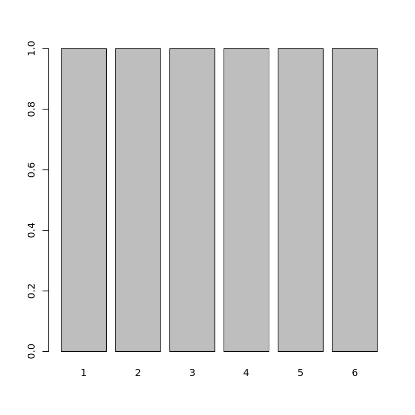
# Plot histogram, hist() doesn't work all the time
barplot(table(list_a))

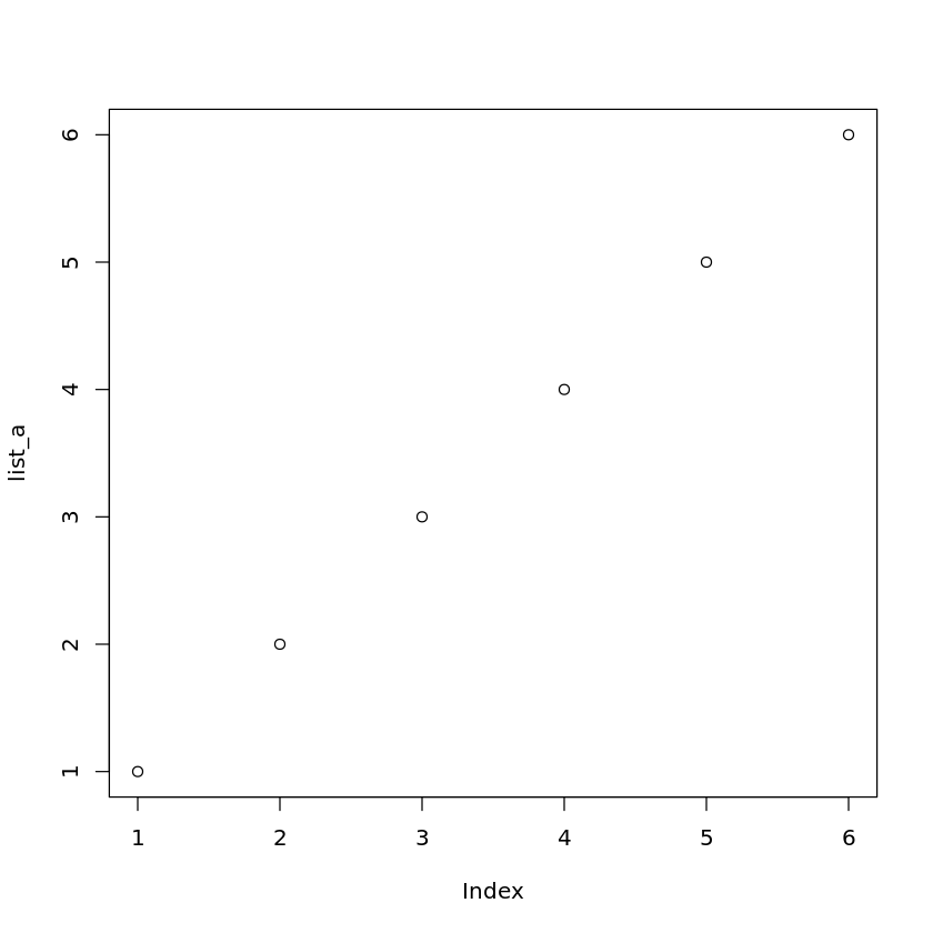
# Plot dot plot
plot(list_a)

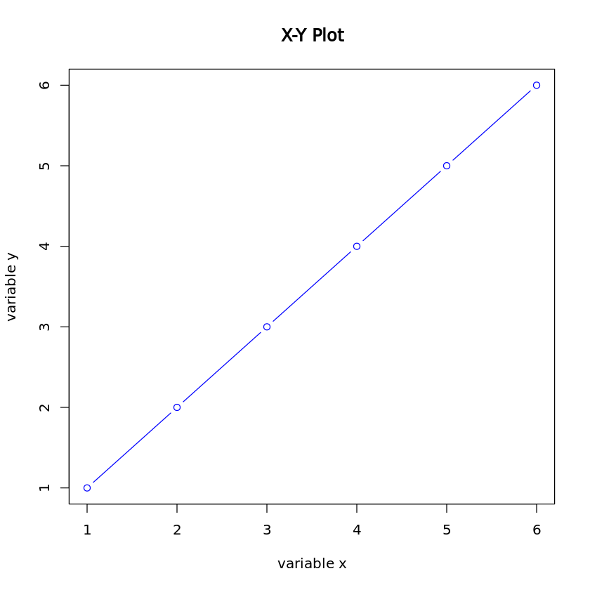
# Plot dot plot
# type: p for point, l for line, b for both
# col: cyan, blue, green, red
plot(list_a, xlab='variable x', ylab='variable y', main='X-Y Plot', type='b', col='blue')

Comments