Convolutional Neural Network with PyTorch

Run Jupyter Notebook

You can run the code for this section in this jupyter notebook link.

About Convolutional Neural Network

Transition From Feedforward Neural Network

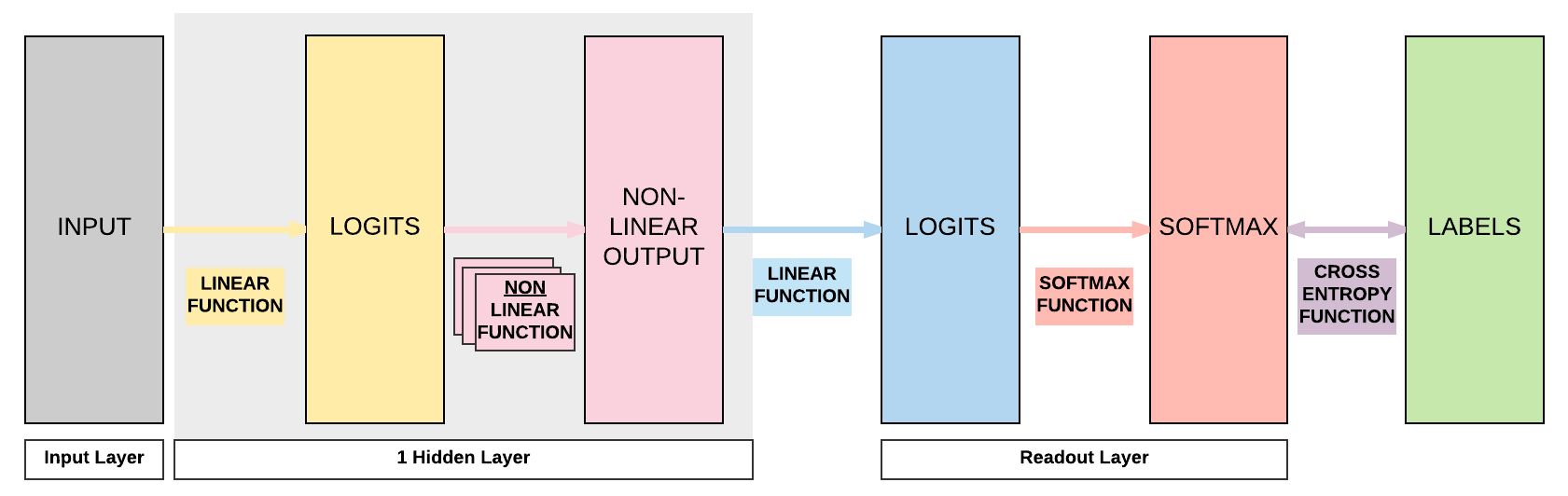
Hidden Layer Feedforward Neural Network

Recap of FNN

So let's do a recap of what we covered in the Feedforward Neural Network (FNN) section using a simple FNN with 1 hidden layer (a pair of affine function and non-linear function)

1. [Yellow box] Pass input into an affine function \(\boldsymbol{y} = A\boldsymbol{x} + \boldsymbol{b}\)
2. [Pink box] Pass logits to non-linear function, for example sigmoid, tanh (hyperbolic tangent), ReLU, or LeakyReLU
3. [Blue box] Pass output of non-linear function to another affine function
4. [Red box] Pass output of final affine function to softmax function to get our probability distribution over K classes
5. [Purple box] Finally we can get our loss by using our cross entropy function

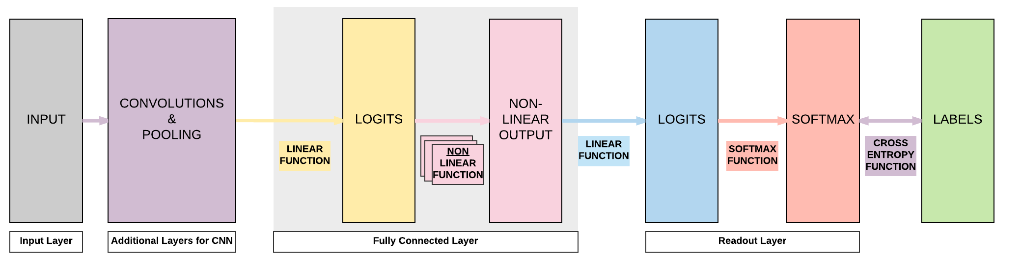
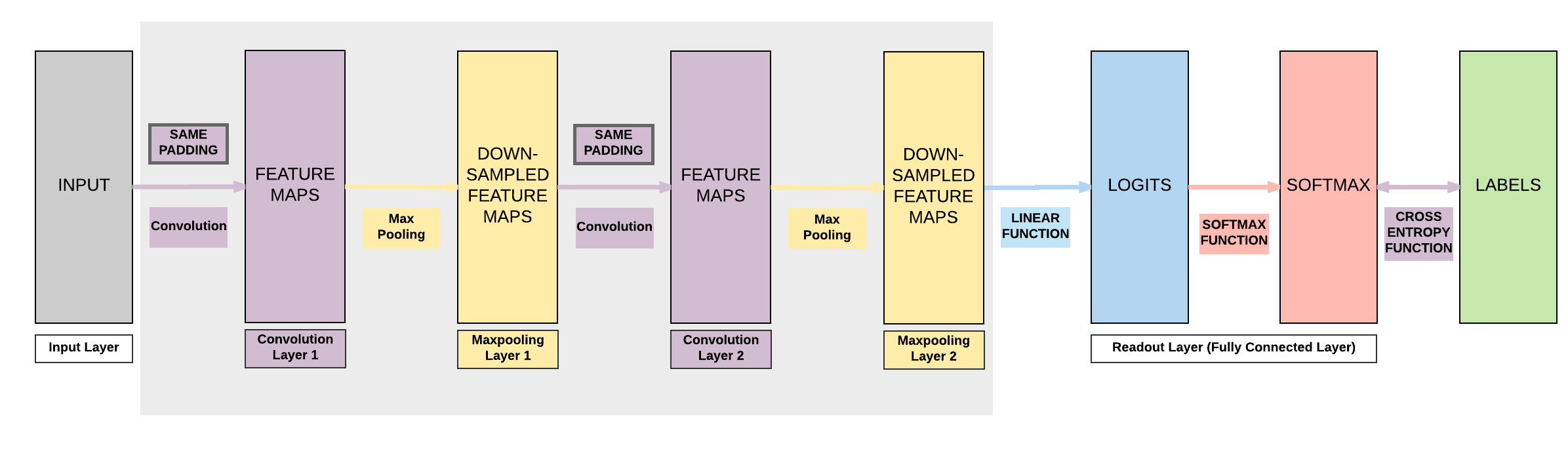
Basic Convolutional Neural Network (CNN)

• A basic CNN just requires 2 additional layers!
  • Convolution and pooling layers before our feedforward neural network

Fully Connected (FC) Layer

A layer with an affine function & non-linear function is called a Fully Connected (FC) layer

One Convolutional Layer: High Level View

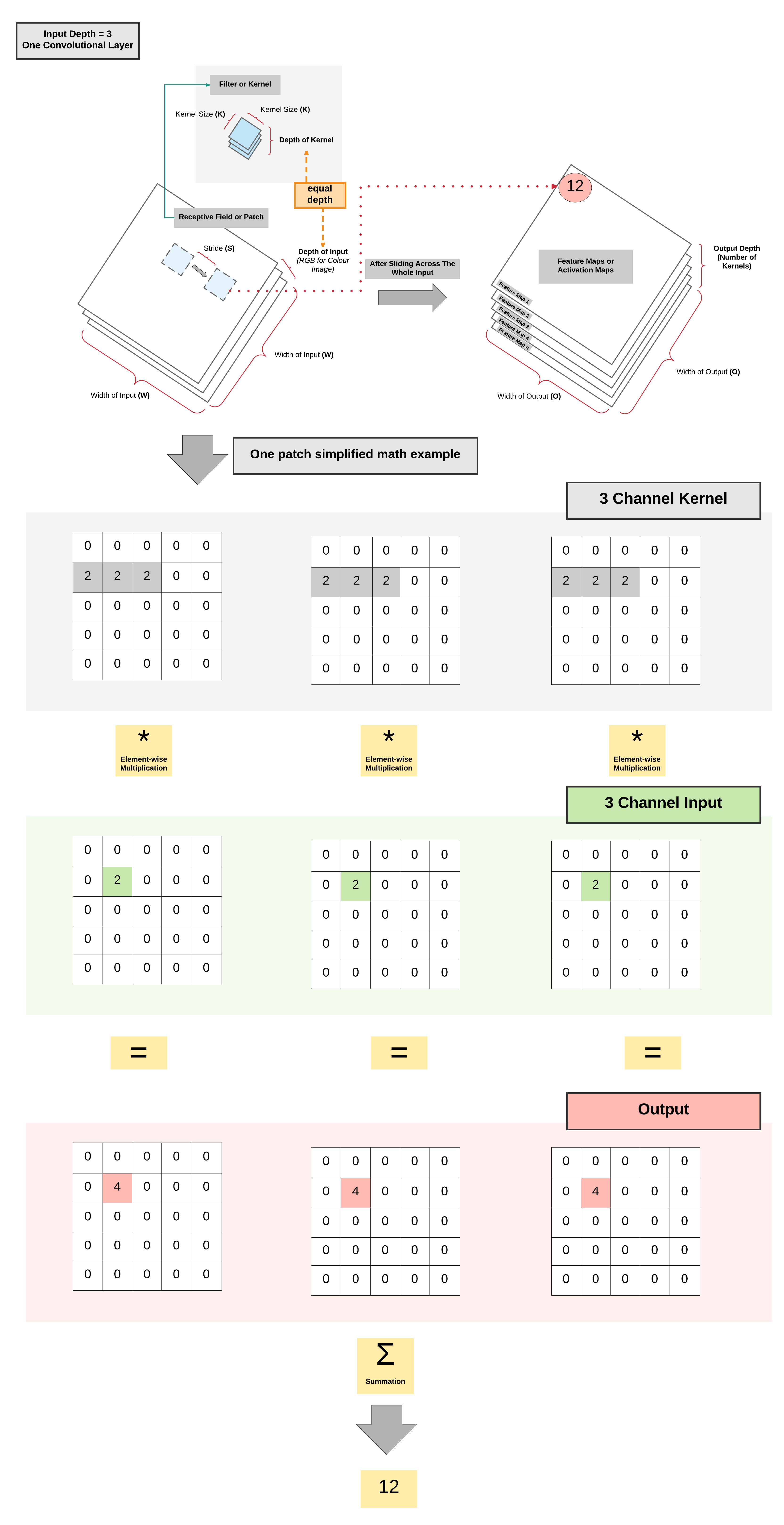
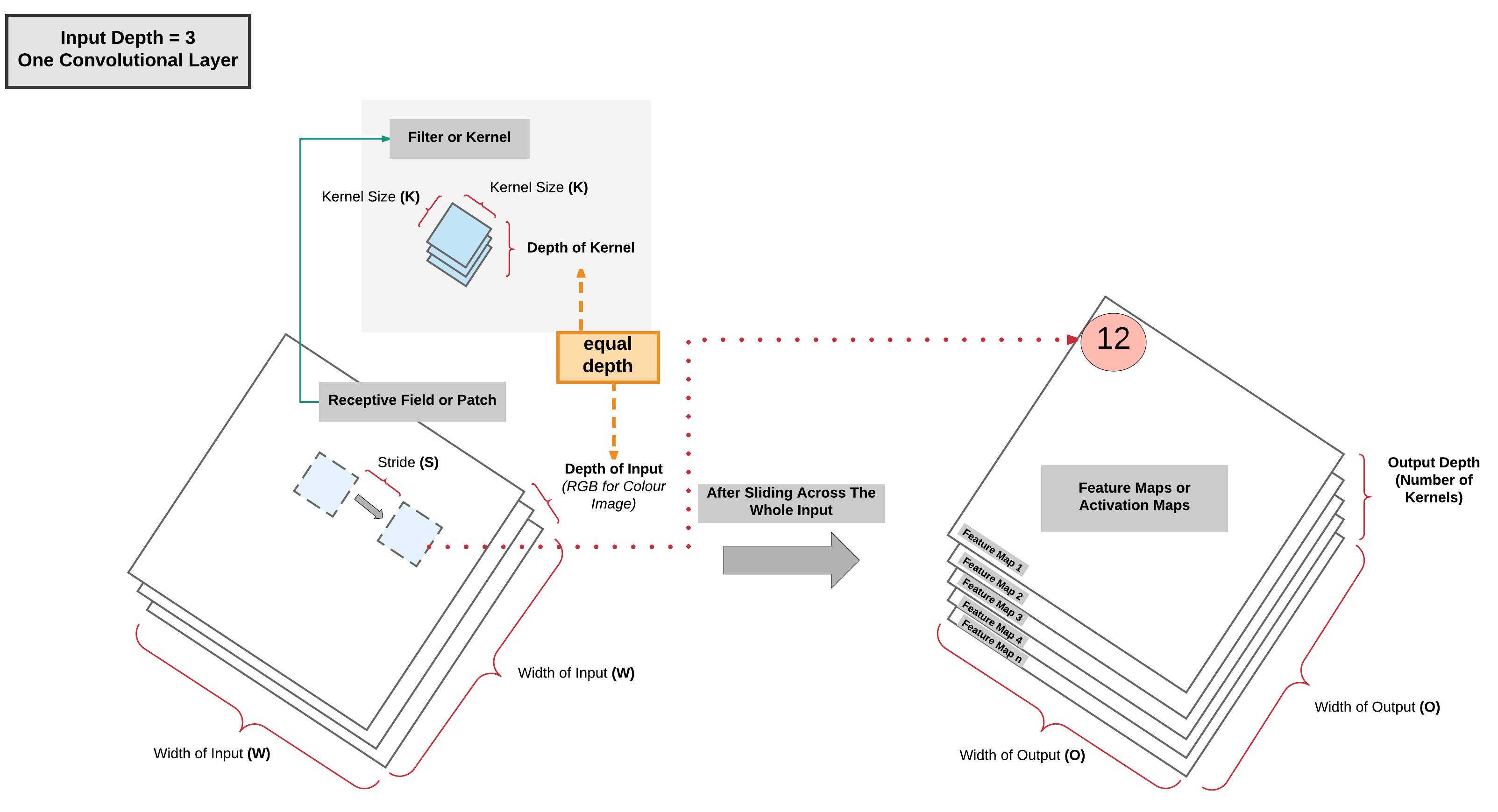
One Convolutional Layer: High Level View Summary

• As the kernel is sliding/convolving across the image \(\rightarrow\) 2 operations done per patch
  1. Element-wise multiplication
  2. Summation
• More kernels \(=\) more feature map channels
  • Can capture more information about the input

Multiple Convolutional Layers: High Level View

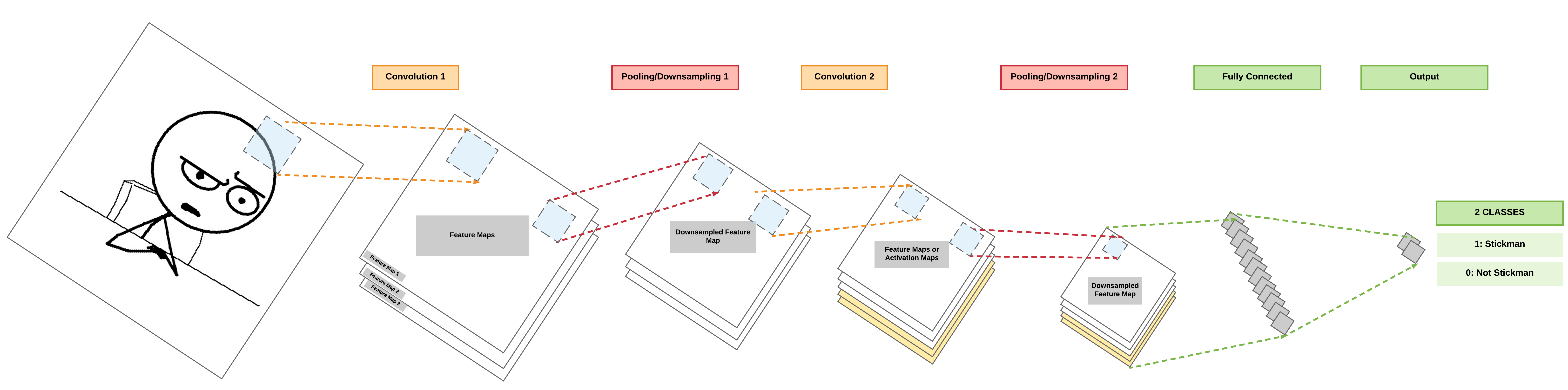
Pooling Layer: High Level View

• 2 Common Types
  • Max Pooling
  • Average Pooling

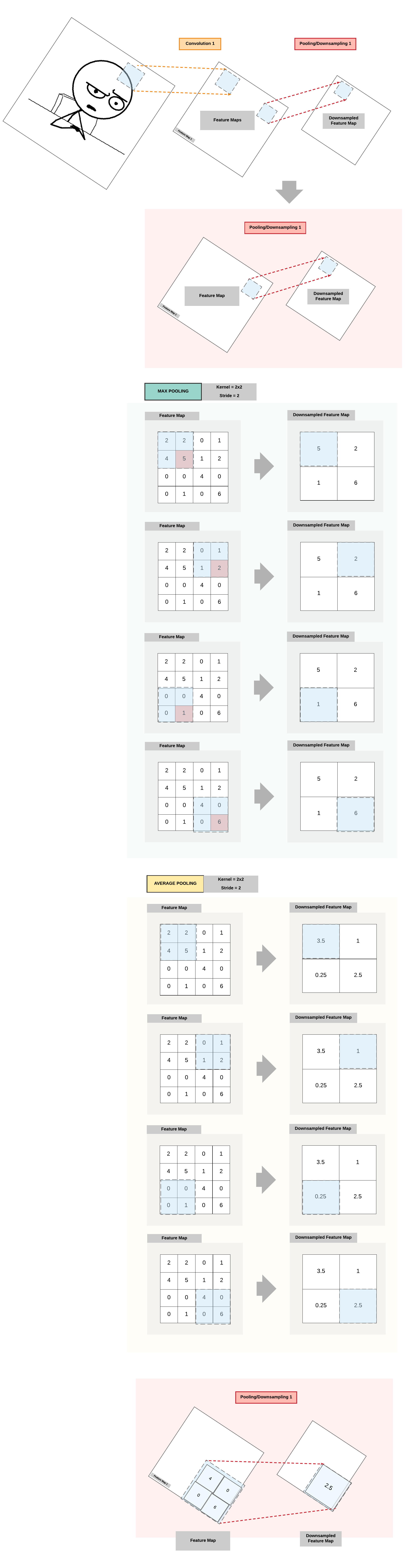
Multiple Pooling Layers: High Level View

Padding

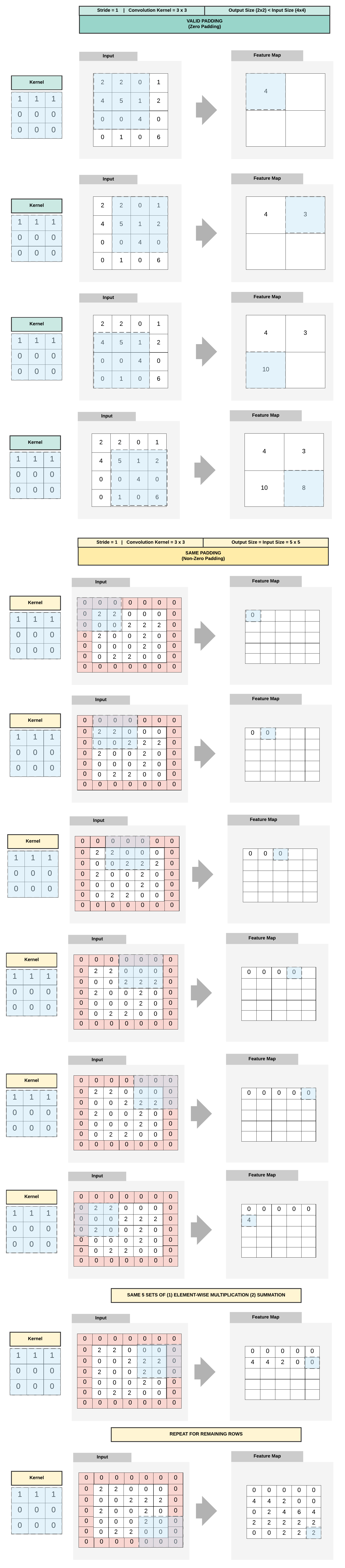
Padding Summary

• Valid Padding (No Padding)
  • Output size < Input Size
• Same Padding (Zero Padding)
  • Output size = Input Size

Dimension Calculations

• \(O = \frac {W - K + 2P}{S} + 1\)
  • \(O\): output height/length
  • \(W\): input height/length
  • \(K\): filter size (kernel size)
  • \(P\): padding
    • \(P = \frac{K - 1}{2}\)
  • \(S\): stride

Example 1: Output Dimension Calculation for Valid Padding

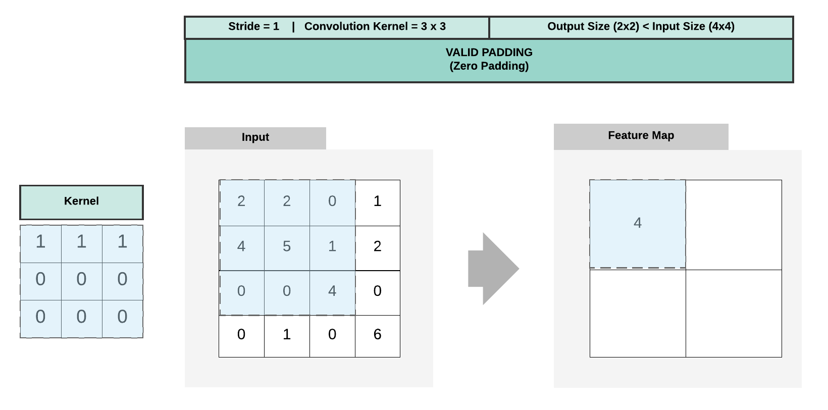
• \(W = 4\)
• \(K = 3\)
• \(P = 0\)
• \(S = 1\)
• \(O = \frac {4 - 3 + 2*0}{1} + 1 = \frac {1}{1} + 1 = 1 + 1 = 2\)

Example 2: Output Dimension Calculation for Same Padding

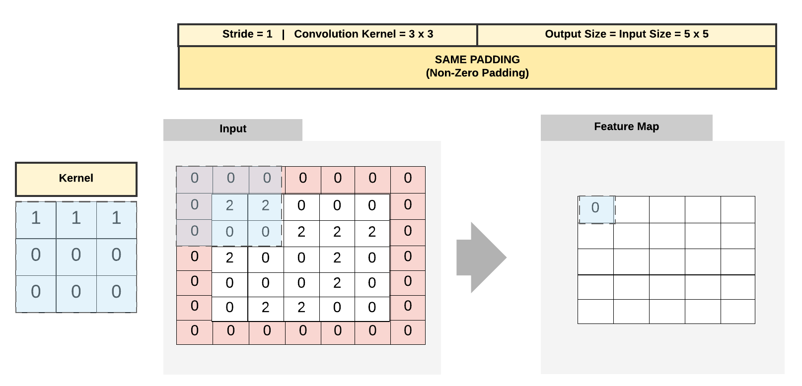
• \(W = 5\)
• \(K = 3\)
• \(P = \frac{3 - 1}{2} = \frac{2}{2} = 1\)
• \(S = 1\)
• \(O = \frac {5 - 3 + 2*1}{1} + 1 = \frac {4}{1} + 1 = 5\)

Building a Convolutional Neural Network with PyTorch

Model A:

• 2 Convolutional Layers
  • Same Padding (same output size)
• 2 Max Pooling Layers
• 1 Fully Connected Layer

Steps

• Step 1: Load Dataset
• Step 2: Make Dataset Iterable
• Step 3: Create Model Class
• Step 4: Instantiate Model Class
• Step 5: Instantiate Loss Class
• Step 6: Instantiate Optimizer Class
• Step 7: Train Model

Step 1: Loading MNIST Train Dataset

Images from 1 to 9

MNIST Dataset and Size of Training Dataset (Excluding Labels)

import torch
import torch.nn as nn
import torchvision.transforms as transforms
import torchvision.datasets as dsets

train_dataset = dsets.MNIST(root='./data', 
                            train=True, 
                            transform=transforms.ToTensor(),
                            download=True)

test_dataset = dsets.MNIST(root='./data', 
                           train=False, 
                           transform=transforms.ToTensor())

print(train_dataset.train_data.size())

torch.Size([60000, 28, 28])

Size of our training dataset labels

print(train_dataset.train_labels.size())

torch.Size([60000])

Size of our testing dataset (excluding labels)

print(test_dataset.test_data.size())

torch.Size([10000, 28, 28])

Size of our testing dataset labels

print(test_dataset.test_labels.size())

torch.Size([10000])

Step 2: Make Dataset Iterable

Load Dataset into Dataloader

batch_size = 100
n_iters = 3000
num_epochs = n_iters / (len(train_dataset) / batch_size)
num_epochs = int(num_epochs)

train_loader = torch.utils.data.DataLoader(dataset=train_dataset, 
                                           batch_size=batch_size, 
                                           shuffle=True)

test_loader = torch.utils.data.DataLoader(dataset=test_dataset, 
                                          batch_size=batch_size, 
                                          shuffle=False)

Step 3: Create Model Class

Output Formula for Convolution

• \(O = \frac {W - K + 2P}{S} + 1\)
  • \(O\): output height/length
  • \(W\): input height/length
  • \(K\): filter size (kernel size) = 5
  • \(P\): same padding (non-zero)
    • \(P = \frac{K - 1}{2} = \frac{5 - 1}{2} = 2\)
  • \(S\): stride = 1

Output Formula for Pooling

• \(O = \frac {W - K}{S} + 1\)
  • W: input height/width
  • K: filter size = 2
  • S: stride size = filter size, PyTorch defaults the stride to kernel filter size
    • If using PyTorch default stride, this will result in the formula \(O = \frac {W}{K}\)
    • By default, in our tutorials, we do this for simplicity.

Define our simple 2 convolutional layer CNN

class CNNModel(nn.Module):
    def __init__(self):
        super(CNNModel, self).__init__()

        # Convolution 1
        self.cnn1 = nn.Conv2d(in_channels=1, out_channels=16, kernel_size=5, stride=1, padding=2)
        self.relu1 = nn.ReLU()

        # Max pool 1
        self.maxpool1 = nn.MaxPool2d(kernel_size=2)

        # Convolution 2
        self.cnn2 = nn.Conv2d(in_channels=16, out_channels=32, kernel_size=5, stride=1, padding=2)
        self.relu2 = nn.ReLU()

        # Max pool 2
        self.maxpool2 = nn.MaxPool2d(kernel_size=2)

        # Fully connected 1 (readout)
        self.fc1 = nn.Linear(32 * 7 * 7, 10) 

    def forward(self, x):
        # Convolution 1
        out = self.cnn1(x)
        out = self.relu1(out)

        # Max pool 1
        out = self.maxpool1(out)

        # Convolution 2 
        out = self.cnn2(out)
        out = self.relu2(out)

        # Max pool 2 
        out = self.maxpool2(out)

        # Resize
        # Original size: (100, 32, 7, 7)
        # out.size(0): 100
        # New out size: (100, 32*7*7)
        out = out.view(out.size(0), -1)

        # Linear function (readout)
        out = self.fc1(out)

        return out

Step 4: Instantiate Model Class

Our model

model = CNNModel()

Step 5: Instantiate Loss Class

• Convolutional Neural Network: Cross Entropy Loss
  • Feedforward Neural Network: Cross Entropy Loss
  • Logistic Regression: Cross Entropy Loss
  • Linear Regression: MSE

Our cross entropy loss

criterion = nn.CrossEntropyLoss()

Step 6: Instantiate Optimizer Class

• Simplified equation
  • \(\theta = \theta - \eta \cdot \nabla_\theta\)
    • \(\theta\): parameters
    • \(\eta\): learning rate (how fast we want to learn)
    • \(\nabla_\theta\): parameters' gradients
• Even simplier equation
  • parameters = parameters - learning_rate * parameters_gradients
  • At every iteration, we update our model's parameters

Optimizer

learning_rate = 0.01

optimizer = torch.optim.SGD(model.parameters(), lr=learning_rate)  

Parameters In-Depth

Print model's parameter

print(model.parameters())

print(len(list(model.parameters())))

# Convolution 1: 16 Kernels
print(list(model.parameters())[0].size())

# Convolution 1 Bias: 16 Kernels
print(list(model.parameters())[1].size())

# Convolution 2: 32 Kernels with depth = 16
print(list(model.parameters())[2].size())

# Convolution 2 Bias: 32 Kernels with depth = 16
print(list(model.parameters())[3].size())

# Fully Connected Layer 1
print(list(model.parameters())[4].size())

# Fully Connected Layer Bias
print(list(model.parameters())[5].size())

<generator object Module.parameters at 0x7f9864363c50>
6
torch.Size([16, 1, 5, 5])
torch.Size([16])
torch.Size([32, 16, 5, 5])
torch.Size([32])
torch.Size([10, 1568])
torch.Size([10])

Step 7: Train Model

• Process
  1. Convert inputs to tensors with gradient accumulation abilities
     • CNN Input: (1, 28, 28)
     • Feedforward NN Input: (1, 28*28)
  2. Clear gradient buffets
  3. Get output given inputs
  4. Get loss
  5. Get gradients w.r.t. parameters
  6. Update parameters using gradients
     • parameters = parameters - learning_rate * parameters_gradients
  7. REPEAT

Model training

iter = 0
for epoch in range(num_epochs):
    for i, (images, labels) in enumerate(train_loader):
        # Load images
        images = images.requires_grad_()

        # Clear gradients w.r.t. parameters
        optimizer.zero_grad()

        # Forward pass to get output/logits
        outputs = model(images)

        # Calculate Loss: softmax --> cross entropy loss
        loss = criterion(outputs, labels)

        # Getting gradients w.r.t. parameters
        loss.backward()

        # Updating parameters
        optimizer.step()

        iter += 1

        if iter % 500 == 0:
            # Calculate Accuracy         
            correct = 0
            total = 0
            # Iterate through test dataset
            for images, labels in test_loader:
                # Load images
                images = images.requires_grad_()

                # Forward pass only to get logits/output
                outputs = model(images)

                # Get predictions from the maximum value
                _, predicted = torch.max(outputs.data, 1)

                # Total number of labels
                total += labels.size(0)

                # Total correct predictions
                correct += (predicted == labels).sum()

            accuracy = 100 * correct / total

            # Print Loss
            print('Iteration: {}. Loss: {}. Accuracy: {}'.format(iter, loss.item(), accuracy))

Iteration: 500. Loss: 0.43324267864227295. Accuracy: 90
Iteration: 1000. Loss: 0.2511480152606964. Accuracy: 92
Iteration: 1500. Loss: 0.13431282341480255. Accuracy: 94
Iteration: 2000. Loss: 0.11173319816589355. Accuracy: 95
Iteration: 2500. Loss: 0.06409914791584015. Accuracy: 96
Iteration: 3000. Loss: 0.14377528429031372. Accuracy: 96

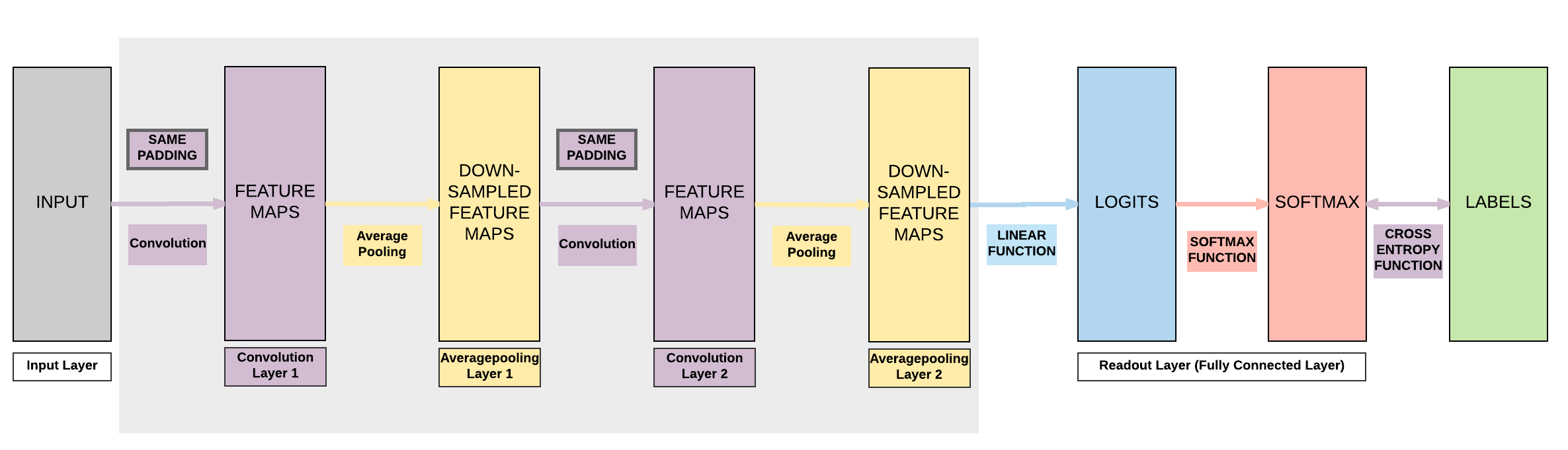
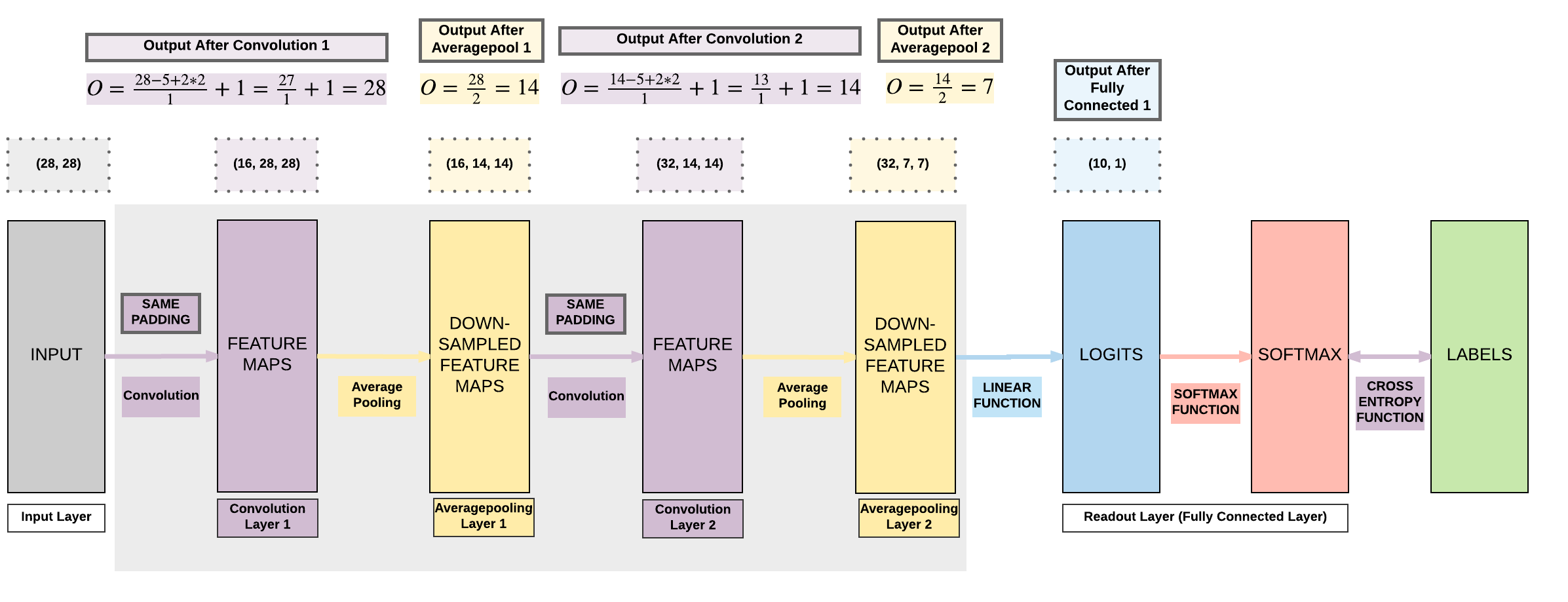
Model B:

• 2 Convolutional Layers
  • Same Padding (same output size)
• 2 Average Pooling Layers
• 1 Fully Connected Layer

Steps

• Step 1: Load Dataset
• Step 2: Make Dataset Iterable
• Step 3: Create Model Class
• Step 4: Instantiate Model Class
• Step 5: Instantiate Loss Class
• Step 6: Instantiate Optimizer Class
• Step 7: Train Model

2 Conv + 2 Average Pool + 1 FC (Zero Padding, Same Padding)

import torch
import torch.nn as nn
import torchvision.transforms as transforms
import torchvision.datasets as dsets

'''
STEP 1: LOADING DATASET
'''

train_dataset = dsets.MNIST(root='./data', 
                            train=True, 
                            transform=transforms.ToTensor(),
                            download=True)

test_dataset = dsets.MNIST(root='./data', 
                           train=False, 
                           transform=transforms.ToTensor())

'''
STEP 2: MAKING DATASET ITERABLE
'''

batch_size = 100
n_iters = 3000
num_epochs = n_iters / (len(train_dataset) / batch_size)
num_epochs = int(num_epochs)

train_loader = torch.utils.data.DataLoader(dataset=train_dataset, 
                                           batch_size=batch_size, 
                                           shuffle=True)

test_loader = torch.utils.data.DataLoader(dataset=test_dataset, 
                                          batch_size=batch_size, 
                                          shuffle=False)

'''
STEP 3: CREATE MODEL CLASS
'''
class CNNModel(nn.Module):
    def __init__(self):
        super(CNNModel, self).__init__()

        # Convolution 1
        self.cnn1 = nn.Conv2d(in_channels=1, out_channels=16, kernel_size=5, stride=1, padding=2)
        self.relu1 = nn.ReLU()

        # Average pool 1
        self.avgpool1 = nn.AvgPool2d(kernel_size=2)

        # Convolution 2
        self.cnn2 = nn.Conv2d(in_channels=16, out_channels=32, kernel_size=5, stride=1, padding=2)
        self.relu2 = nn.ReLU()

        # Average pool 2
        self.avgpool2 = nn.AvgPool2d(kernel_size=2)

        # Fully connected 1 (readout)
        self.fc1 = nn.Linear(32 * 7 * 7, 10) 

    def forward(self, x):
        # Convolution 1
        out = self.cnn1(x)
        out = self.relu1(out)

        # Average pool 1
        out = self.avgpool1(out)

        # Convolution 2 
        out = self.cnn2(out)
        out = self.relu2(out)

        # Max pool 2 
        out = self.avgpool2(out)

        # Resize
        # Original size: (100, 32, 7, 7)
        # out.size(0): 100
        # New out size: (100, 32*7*7)
        out = out.view(out.size(0), -1)

        # Linear function (readout)
        out = self.fc1(out)

        return out

'''
STEP 4: INSTANTIATE MODEL CLASS
'''

model = CNNModel()

'''
STEP 5: INSTANTIATE LOSS CLASS
'''
criterion = nn.CrossEntropyLoss()


'''
STEP 6: INSTANTIATE OPTIMIZER CLASS
'''
learning_rate = 0.01

optimizer = torch.optim.SGD(model.parameters(), lr=learning_rate)

'''
STEP 7: TRAIN THE MODEL
'''
iter = 0
for epoch in range(num_epochs):
    for i, (images, labels) in enumerate(train_loader):
        # Load images as tensors with gradient accumulation abilities
        images = images.requires_grad_()

        # Clear gradients w.r.t. parameters
        optimizer.zero_grad()

        # Forward pass to get output/logits
        outputs = model(images)

        # Calculate Loss: softmax --> cross entropy loss
        loss = criterion(outputs, labels)

        # Getting gradients w.r.t. parameters
        loss.backward()

        # Updating parameters
        optimizer.step()

        iter += 1

        if iter % 500 == 0:
            # Calculate Accuracy         
            correct = 0
            total = 0
            # Iterate through test dataset
            for images, labels in test_loader:
                # Load images to tensors with gradient accumulation abilities
                images = images.requires_grad_()

                # Forward pass only to get logits/output
                outputs = model(images)

                # Get predictions from the maximum value
                _, predicted = torch.max(outputs.data, 1)

                # Total number of labels
                total += labels.size(0)

                # Total correct predictions
                correct += (predicted == labels).sum()

            accuracy = 100 * correct / total

            # Print Loss
            print('Iteration: {}. Loss: {}. Accuracy: {}'.format(iter, loss.item(), accuracy))

Iteration: 500. Loss: 0.6850348711013794. Accuracy: 85
Iteration: 1000. Loss: 0.36549052596092224. Accuracy: 88
Iteration: 1500. Loss: 0.31540098786354065. Accuracy: 89
Iteration: 2000. Loss: 0.3522164225578308. Accuracy: 90
Iteration: 2500. Loss: 0.2680729925632477. Accuracy: 91
Iteration: 3000. Loss: 0.26440390944480896. Accuracy: 92

Comparison of accuracies

It seems like average pooling test accuracy is less than the max pooling accuracy! Does this mean average pooling is better? This is not definitive and depends on a lot of factors including the model's architecture, seed (that affects random weight initialization) and more.

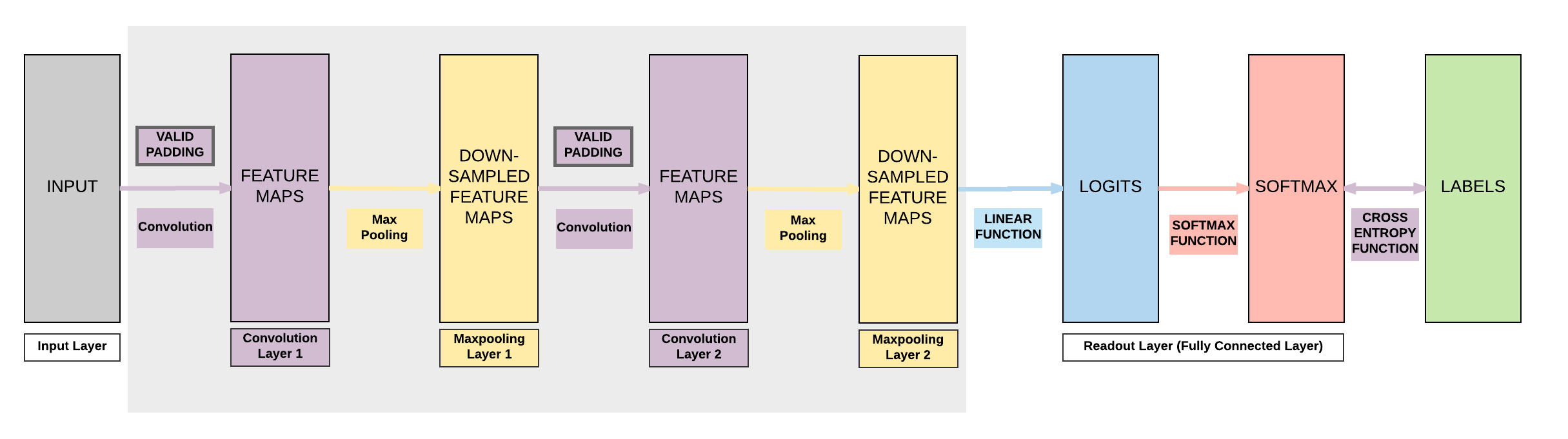
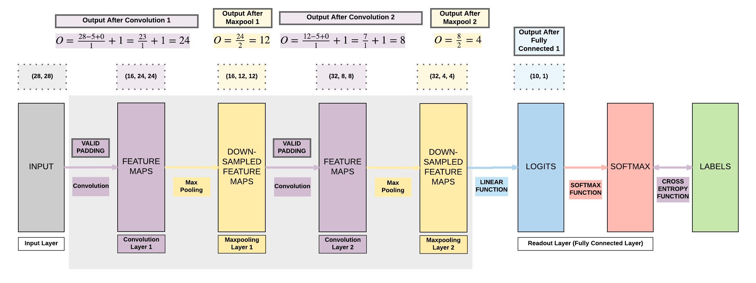
Model C:

• 2 Convolutional Layers
  • Valid Padding (smaller output size)
• 2 Max Pooling Layers
• 1 Fully Connected Layer

Steps

• Step 1: Load Dataset
• Step 2: Make Dataset Iterable
• Step 3: Create Model Class
• Step 4: Instantiate Model Class
• Step 5: Instantiate Loss Class
• Step 6: Instantiate Optimizer Class
• Step 7: Train Model

2 Conv + 2 Max Pool + 1 FC (Valid Padding, No Padding)

import torch
import torch.nn as nn
import torchvision.transforms as transforms
import torchvision.datasets as dsets

'''
STEP 1: LOADING DATASET
'''

train_dataset = dsets.MNIST(root='./data', 
                            train=True, 
                            transform=transforms.ToTensor(),
                            download=True)

test_dataset = dsets.MNIST(root='./data', 
                           train=False, 
                           transform=transforms.ToTensor())

'''
STEP 2: MAKING DATASET ITERABLE
'''

batch_size = 100
n_iters = 3000
num_epochs = n_iters / (len(train_dataset) / batch_size)
num_epochs = int(num_epochs)

train_loader = torch.utils.data.DataLoader(dataset=train_dataset, 
                                           batch_size=batch_size, 
                                           shuffle=True)

test_loader = torch.utils.data.DataLoader(dataset=test_dataset, 
                                          batch_size=batch_size, 
                                          shuffle=False)

'''
STEP 3: CREATE MODEL CLASS
'''
class CNNModel(nn.Module):
    def __init__(self):
        super(CNNModel, self).__init__()

        # Convolution 1
        self.cnn1 = nn.Conv2d(in_channels=1, out_channels=16, kernel_size=5, stride=1, padding=0)
        self.relu1 = nn.ReLU()

        # Max pool 1
        self.maxpool1 = nn.MaxPool2d(kernel_size=2)

        # Convolution 2
        self.cnn2 = nn.Conv2d(in_channels=16, out_channels=32, kernel_size=5, stride=1, padding=0)
        self.relu2 = nn.ReLU()

        # Max pool 2
        self.maxpool2 = nn.MaxPool2d(kernel_size=2)

        # Fully connected 1 (readout)
        self.fc1 = nn.Linear(32 * 4 * 4, 10) 

    def forward(self, x):
        # Convolution 1
        out = self.cnn1(x)
        out = self.relu1(out)

        # Max pool 1
        out = self.maxpool1(out)

        # Convolution 2 
        out = self.cnn2(out)
        out = self.relu2(out)

        # Max pool 2 
        out = self.maxpool2(out)

        # Resize
        # Original size: (100, 32, 7, 7)
        # out.size(0): 100
        # New out size: (100, 32*7*7)
        out = out.view(out.size(0), -1)

        # Linear function (readout)
        out = self.fc1(out)

        return out

'''
STEP 4: INSTANTIATE MODEL CLASS
'''

model = CNNModel()

'''
STEP 5: INSTANTIATE LOSS CLASS
'''
criterion = nn.CrossEntropyLoss()


'''
STEP 6: INSTANTIATE OPTIMIZER CLASS
'''
learning_rate = 0.01

optimizer = torch.optim.SGD(model.parameters(), lr=learning_rate)

'''
STEP 7: TRAIN THE MODEL
'''
iter = 0
for epoch in range(num_epochs):
    for i, (images, labels) in enumerate(train_loader):
        # Load images as tensors with gradient accumulation abilities
        images = images.requires_grad_()

        # Clear gradients w.r.t. parameters
        optimizer.zero_grad()

        # Forward pass to get output/logits
        outputs = model(images)

        # Calculate Loss: softmax --> cross entropy loss
        loss = criterion(outputs, labels)

        # Getting gradients w.r.t. parameters
        loss.backward()

        # Updating parameters
        optimizer.step()

        iter += 1

        if iter % 500 == 0:
            # Calculate Accuracy         
            correct = 0
            total = 0
            # Iterate through test dataset
            for images, labels in test_loader:
                # Load images to tensors with gradient accumulation abilities
                images = images.requires_grad_()

                # Forward pass only to get logits/output
                outputs = model(images)

                # Get predictions from the maximum value
                _, predicted = torch.max(outputs.data, 1)

                # Total number of labels
                total += labels.size(0)

                # Total correct predictions
                correct += (predicted == labels).sum()

            accuracy = 100 * correct / total

            # Print Loss
            print('Iteration: {}. Loss: {}. Accuracy: {}'.format(iter, loss.item(), accuracy))

Iteration: 500. Loss: 0.5153220295906067. Accuracy: 88
Iteration: 1000. Loss: 0.28784745931625366. Accuracy: 92
Iteration: 1500. Loss: 0.4086027443408966. Accuracy: 94
Iteration: 2000. Loss: 0.09390712529420853. Accuracy: 95
Iteration: 2500. Loss: 0.07138358801603317. Accuracy: 95
Iteration: 3000. Loss: 0.05396252125501633. Accuracy: 96

Summary of Results

Model A	Model B	Model C
Max Pooling	Average Pooling	Max Pooling
Same Padding	Same Padding	Valid Padding
97.04%	93.59%	96.5%

All Models
INPUT \(\rightarrow\) CONV \(\rightarrow\) POOL \(\rightarrow\) CONV \(\rightarrow\) POOL \(\rightarrow\) FC
Convolution Kernel Size = 5 x 5
Convolution Kernel Stride = 1
Pooling Kernel Size = 2 x 2

General Deep Learning Notes on CNN and FNN

• 3 ways to expand a convolutional neural network
  • More convolutional layers
  • Less aggressive downsampling
    • Smaller kernel size for pooling (gradually downsampling)
  • More fully connected layers
• Cons
  • Need a larger dataset
    • Curse of dimensionality
  • Does not necessarily mean higher accuracy

3. Building a Convolutional Neural Network with PyTorch (GPU)

Model A

GPU: 2 things must be on GPU - model - tensors

Steps

• Step 1: Load Dataset
• Step 2: Make Dataset Iterable
• Step 3: Create Model Class
• Step 4: Instantiate Model Class
• Step 5: Instantiate Loss Class
• Step 6: Instantiate Optimizer Class
• Step 7: Train Model

2 Conv + 2 Max Pooling + 1 FC (Same Padding, Zero Padding)

import torch
import torch.nn as nn
import torchvision.transforms as transforms
import torchvision.datasets as dsets 

'''
STEP 1: LOADING DATASET
'''

train_dataset = dsets.MNIST(root='./data', 
                            train=True, 
                            transform=transforms.ToTensor(),
                            download=True)

test_dataset = dsets.MNIST(root='./data', 
                           train=False, 
                           transform=transforms.ToTensor())

'''
STEP 2: MAKING DATASET ITERABLE
'''

batch_size = 100
n_iters = 3000
num_epochs = n_iters / (len(train_dataset) / batch_size)
num_epochs = int(num_epochs)

train_loader = torch.utils.data.DataLoader(dataset=train_dataset, 
                                           batch_size=batch_size, 
                                           shuffle=True)

test_loader = torch.utils.data.DataLoader(dataset=test_dataset, 
                                          batch_size=batch_size, 
                                          shuffle=False)

'''
STEP 3: CREATE MODEL CLASS
'''
class CNNModel(nn.Module):
    def __init__(self):
        super(CNNModel, self).__init__()

        # Convolution 1
        self.cnn1 = nn.Conv2d(in_channels=1, out_channels=16, kernel_size=5, stride=1, padding=0)
        self.relu1 = nn.ReLU()

        # Max pool 1
        self.maxpool1 = nn.MaxPool2d(kernel_size=2)

        # Convolution 2
        self.cnn2 = nn.Conv2d(in_channels=16, out_channels=32, kernel_size=5, stride=1, padding=0)
        self.relu2 = nn.ReLU()

        # Max pool 2
        self.maxpool2 = nn.MaxPool2d(kernel_size=2)

        # Fully connected 1 (readout)
        self.fc1 = nn.Linear(32 * 4 * 4, 10) 

    def forward(self, x):
        # Convolution 1
        out = self.cnn1(x)
        out = self.relu1(out)

        # Max pool 1
        out = self.maxpool1(out)

        # Convolution 2 
        out = self.cnn2(out)
        out = self.relu2(out)

        # Max pool 2 
        out = self.maxpool2(out)

        # Resize
        # Original size: (100, 32, 7, 7)
        # out.size(0): 100
        # New out size: (100, 32*7*7)
        out = out.view(out.size(0), -1)

        # Linear function (readout)
        out = self.fc1(out)

        return out

'''
STEP 4: INSTANTIATE MODEL CLASS
'''

model = CNNModel()

#######################
#  USE GPU FOR MODEL  #
#######################

device = torch.device("cuda:0" if torch.cuda.is_available() else "cpu")
model.to(device)

'''
STEP 5: INSTANTIATE LOSS CLASS
'''
criterion = nn.CrossEntropyLoss()


'''
STEP 6: INSTANTIATE OPTIMIZER CLASS
'''
learning_rate = 0.01

optimizer = torch.optim.SGD(model.parameters(), lr=learning_rate)

'''
STEP 7: TRAIN THE MODEL
'''
iter = 0
for epoch in range(num_epochs):
    for i, (images, labels) in enumerate(train_loader):

        #######################
        #  USE GPU FOR MODEL  #
        #######################
        images = images.requires_grad_().to(device)
        labels = labels.to(device)

        # Clear gradients w.r.t. parameters
        optimizer.zero_grad()

        # Forward pass to get output/logits
        outputs = model(images)

        # Calculate Loss: softmax --> cross entropy loss
        loss = criterion(outputs, labels)

        # Getting gradients w.r.t. parameters
        loss.backward()

        # Updating parameters
        optimizer.step()

        iter += 1

        if iter % 500 == 0:
            # Calculate Accuracy         
            correct = 0
            total = 0
            # Iterate through test dataset
            for images, labels in test_loader:
                #######################
                #  USE GPU FOR MODEL  #
                #######################
                images = images.requires_grad_().to(device)
                labels = labels.to(device)

                # Forward pass only to get logits/output
                outputs = model(images)

                # Get predictions from the maximum value
                _, predicted = torch.max(outputs.data, 1)

                # Total number of labels
                total += labels.size(0)

                #######################
                #  USE GPU FOR MODEL  #
                #######################
                # Total correct predictions
                if torch.cuda.is_available():
                    correct += (predicted.cpu() == labels.cpu()).sum()
                else:
                    correct += (predicted == labels).sum()

            accuracy = 100 * correct / total

            # Print Loss
            print('Iteration: {}. Loss: {}. Accuracy: {}'.format(iter, loss.item(), accuracy))

Iteration: 500. Loss: 0.36831170320510864. Accuracy: 88
Iteration: 1000. Loss: 0.31790846586227417. Accuracy: 92
Iteration: 1500. Loss: 0.1510857343673706. Accuracy: 94
Iteration: 2000. Loss: 0.08368007838726044. Accuracy: 95
Iteration: 2500. Loss: 0.13419771194458008. Accuracy: 96
Iteration: 3000. Loss: 0.16750787198543549. Accuracy: 96

More Efficient Convolutions via Toeplitz Matrices

This is beyond the scope of this particular lesson. But now that we understand how convolutions work, it is critical to know that it is quite an inefficient operation if we use for-loops to perform our 2D convolutions (5 x 5 convolution kernel size for example) on our 2D images (28 x 28 MNIST image for example).

A more efficient implementation is in converting our convolution kernel into a doubly block circulant/Toeplitz matrix (special case Toeplitz matrix) and our image (input) into a vector. Then, we will do just one matrix operation using our doulby block Toeplitz matrix and our input vector.

There will be a whole lesson dedicated to this operation released down the road.

Summary

We've learnt to...

Success

• Transition from Feedforward Neural Network
  • Addition of Convolutional & Pooling Layers before Linear Layers
• One Convolutional Layer Basics
• One Pooling Layer Basics
  • Max pooling
  • Average pooling
• Padding
• Output Dimension Calculations and Examples
  • \(O = \frac {W - K + 2P}{S} + 1\)
• Convolutional Neural Networks
  • Model A: 2 Conv + 2 Max pool + 1 FC
    • Same Padding
  • Model B: 2 Conv + 2 Average pool + 1 FC
    • Same Padding
  • Model C: 2 Conv + 2 Max pool + 1 FC
    • Valid Padding
• Model Variation in Code
  • Modifying only step 3
• Ways to Expand Model’s Capacity
  • More convolutions
  • Gradual pooling
  • More fully connected layers
• GPU Code
  • 2 things on GPU
    • model
    • tensors with gradient accumulation abilities
  • Modifying only Step 4 & Step 7
• 7 Step Model Building Recap
  • Step 1: Load Dataset
  • Step 2: Make Dataset Iterable
  • Step 3: Create Model Class
  • Step 4: Instantiate Model Class
  • Step 5: Instantiate Loss Class
  • Step 6: Instantiate Optimizer Class
  • Step 7: Train Model

Citation

If you have found these useful in your research, presentations, school work, projects or workshops, feel free to cite using this DOI.

Comments